Gallery#

This section shows example plots produced by ESMValTool. For more information, follow the links in the figure captions.A website displaying results produced with the latest release of ESMValTool for all available recipes can be accessed here.

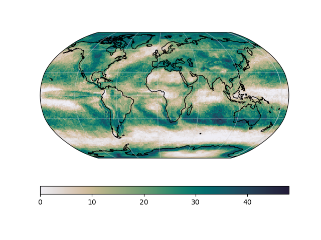
_images/consec_example_freq.png — Fig. 2 Example of the number of occurrences with consecutive dry days of more than five days in the period …#

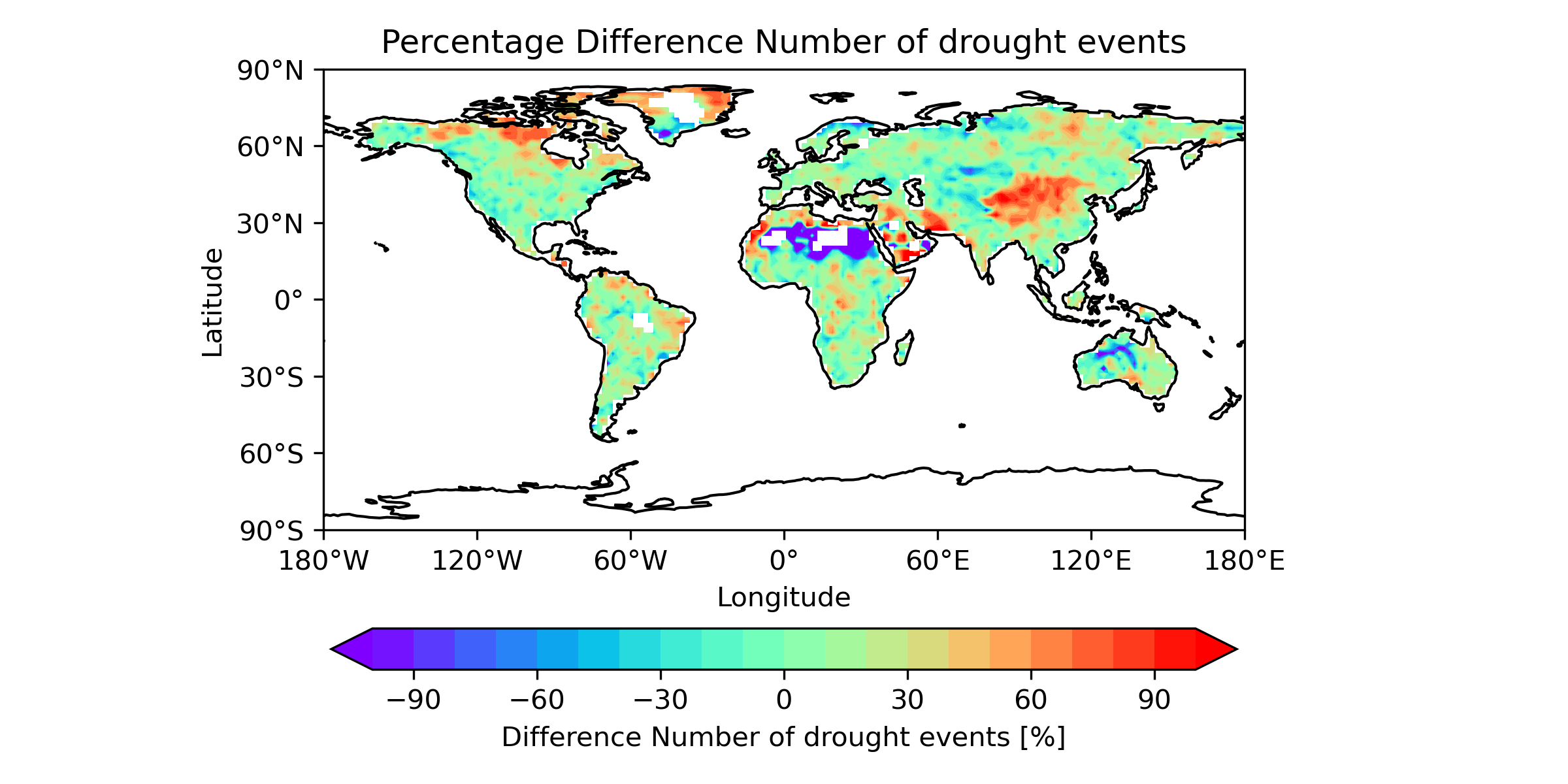
_images/martin18grl_fig1.png — Fig. 3 Global map of the percentage difference between multi-model mean of 15 CMIP models and the CRU data …#

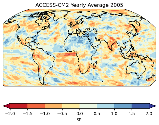
_images/spi_example.png — Fig. 4 Example plot of SPI averaged over the year 2005. The reference period for index calibration is 2000-…#

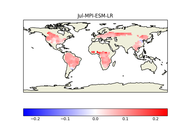
_images/MPI-ESM-LR_albedo_change_from_tree_to_crop-grass.png — Fig. 5 Example of albedo change from tree to crop and grass for the CMIP5 model MPI-ESM-LR derived for the …#

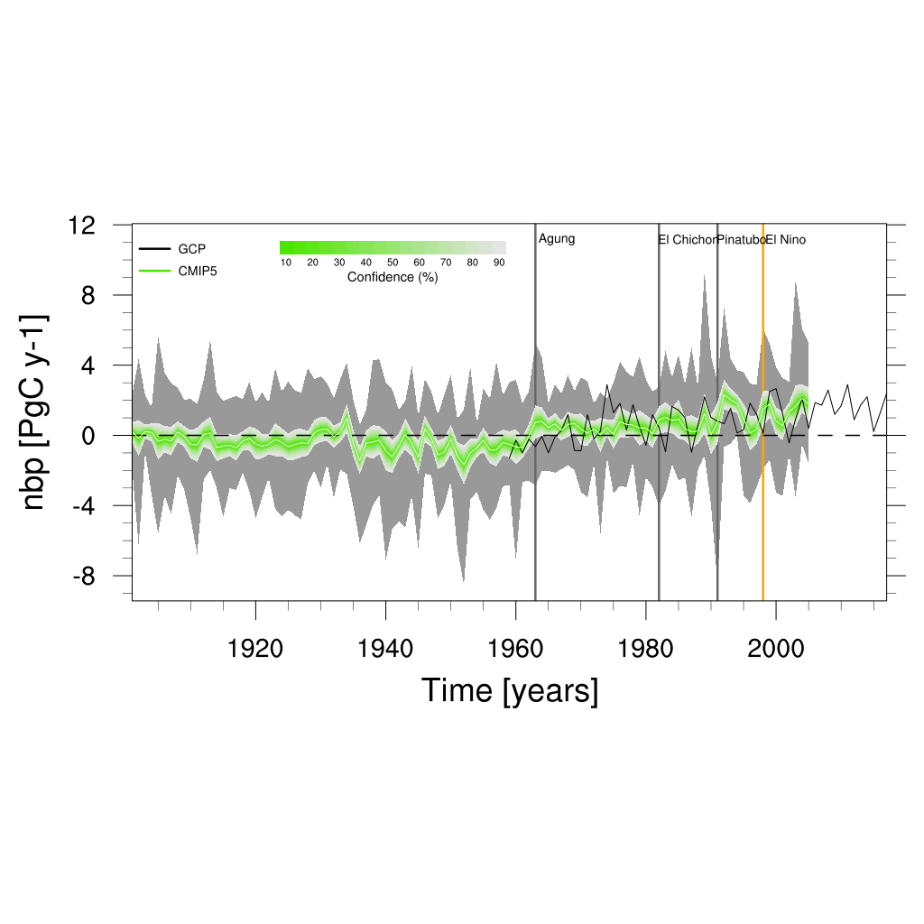
_images/nbp_evolution_global.png — Fig. 6 Time series of global net biome productivity (NBP) over the period 1901-2005. Similar to Anav et al….#

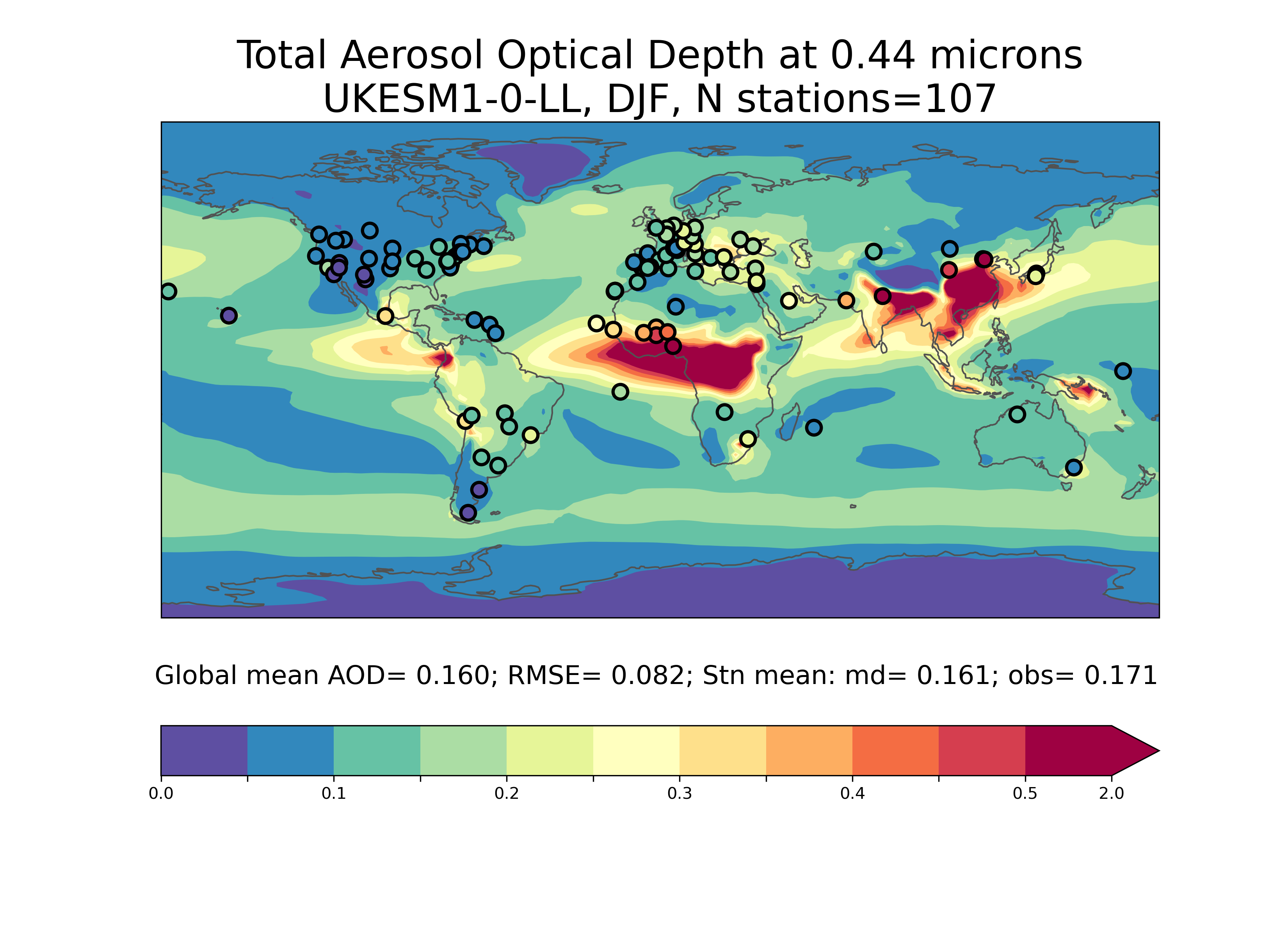
_images/UKESM1-0-LL_CMIP_AERmon_historical_od440aer_gn_1994_2014_DJF.png — Fig. 7 Evaluation of AOD at 440 nm from UKESM1 historical ensemble member r1i1p1f2 against the AeroNET clim…#

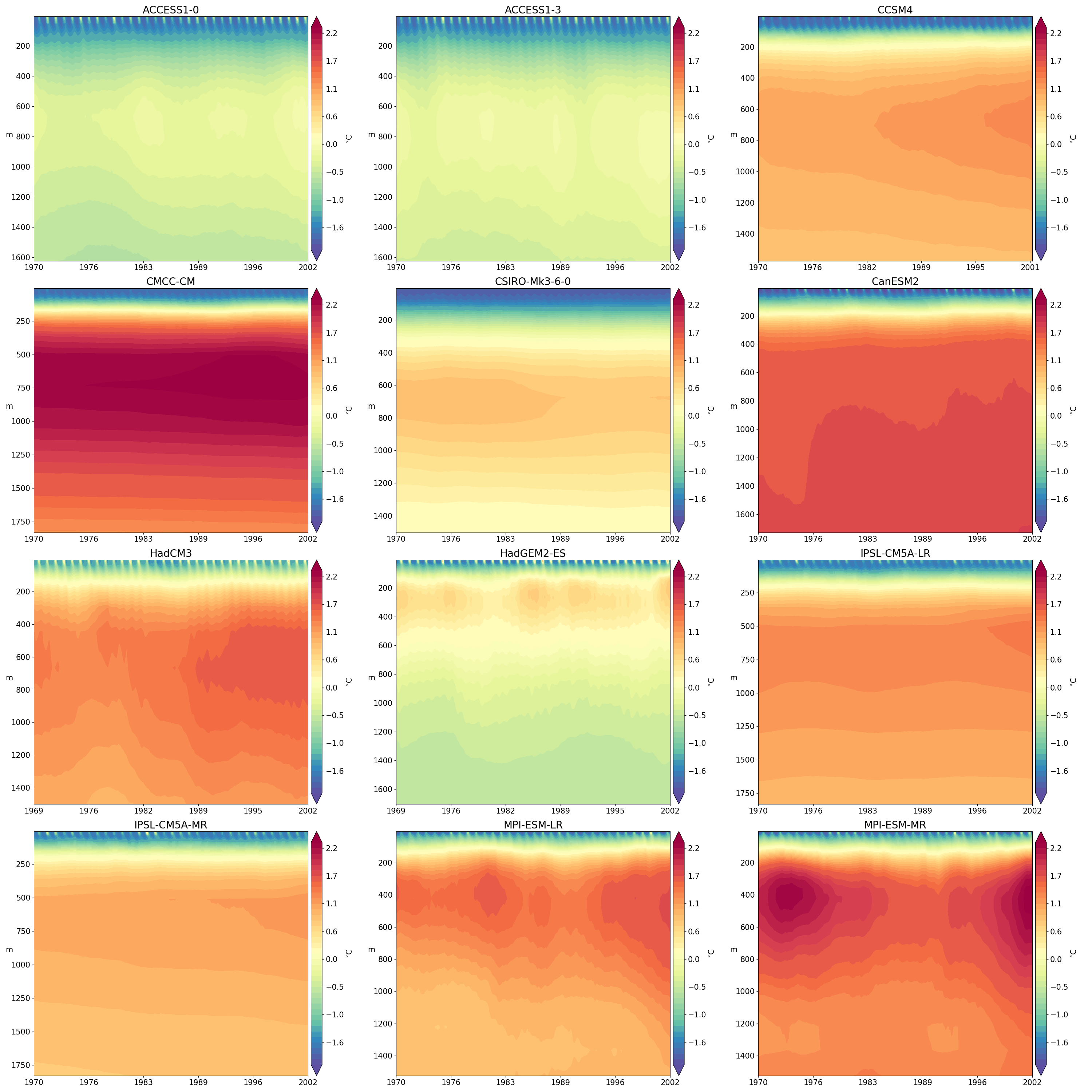
_images/hofm.png — Fig. 8 Hovmoller diagram of monthly spatially averaged potential temperature in the Eurasian Basin of the A…#

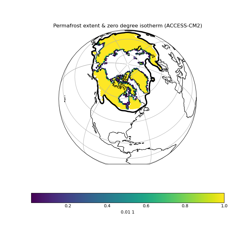
_images/pf_extent_north_america_ACCESS-CM2.png — Fig. 9 Permafrost extent and zero degC isotherm, showing North America#

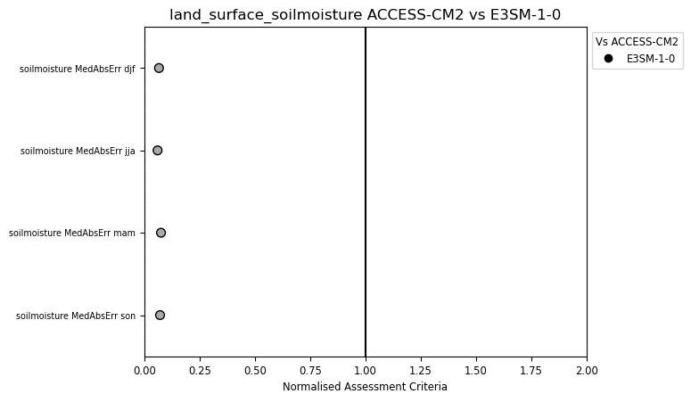
_images/Soilmoisture_Metrics.png — Fig. 10 Normalised metrics plot comparing a control and experiment simulation#

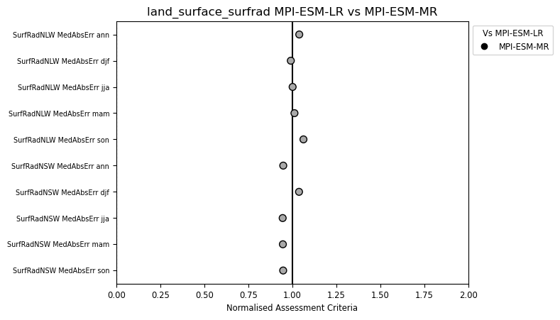
_images/Surfrad_Metrics.png — Fig. 11 Normalised metrics plot comparing a control and experiment simulation#

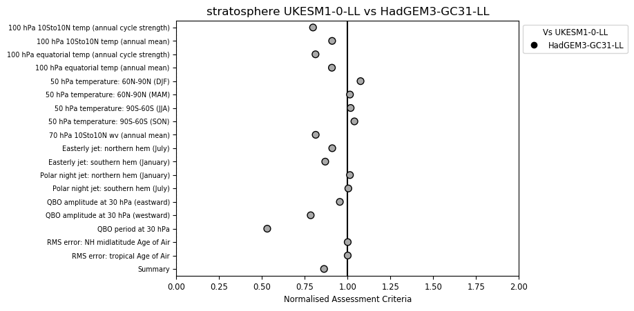
_images/metrics.png — Fig. 12 Standard metrics plot comparing standard metrics from UKESM1-0-LL and HadGEM3-GC31.#

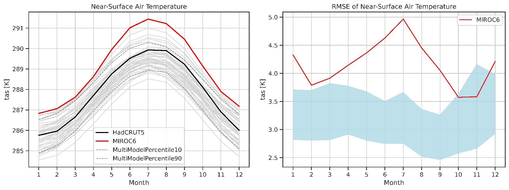
_images/annual_cycle.png — Fig. 13 (Left) Multi-year global mean (2000-2004) of the seasonal cycle of near-surface temperature in K fro…#

_images/tas_Global_CMIP6_historical_anom_1850-2014.png — Fig. 14 Observed and simulated time series of the anomalies in annual and global mean surface temperature. A…#

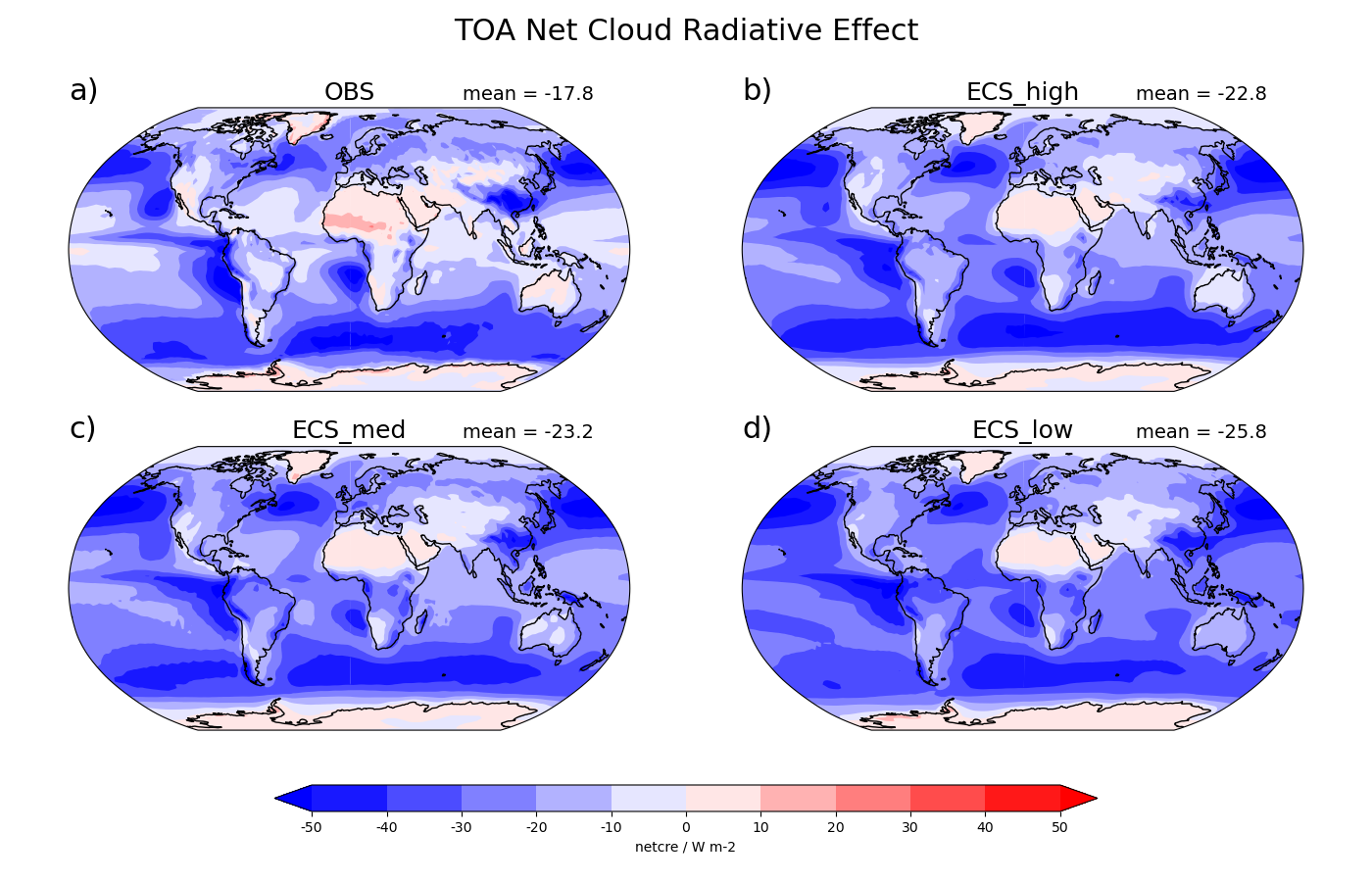
_images/map_netcre.png — Fig. 15 Geographical map of the multi-year annual mean net cloud radiative effect from (a) CERES–EBAF Ed4.2 …#

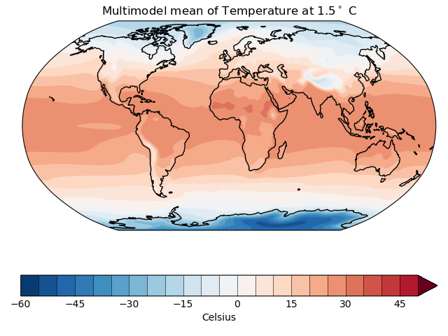
_images/CMIP6_mm_mean_ssp126_1.5_tas.png — Fig. 16 Multimodel mean of temperature under SSP1-2.6 at 1.5 degC warming.#

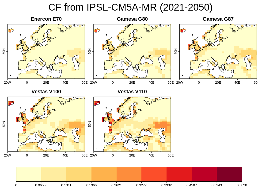
_images/capacity_factor_IPSL-CM5A-MR_2021-2050.png — Fig. 17 Wind capacity factor for five turbines: Enercon E70 (top-left), Gamesa G80 (middle-top), Gamesa G87 …#

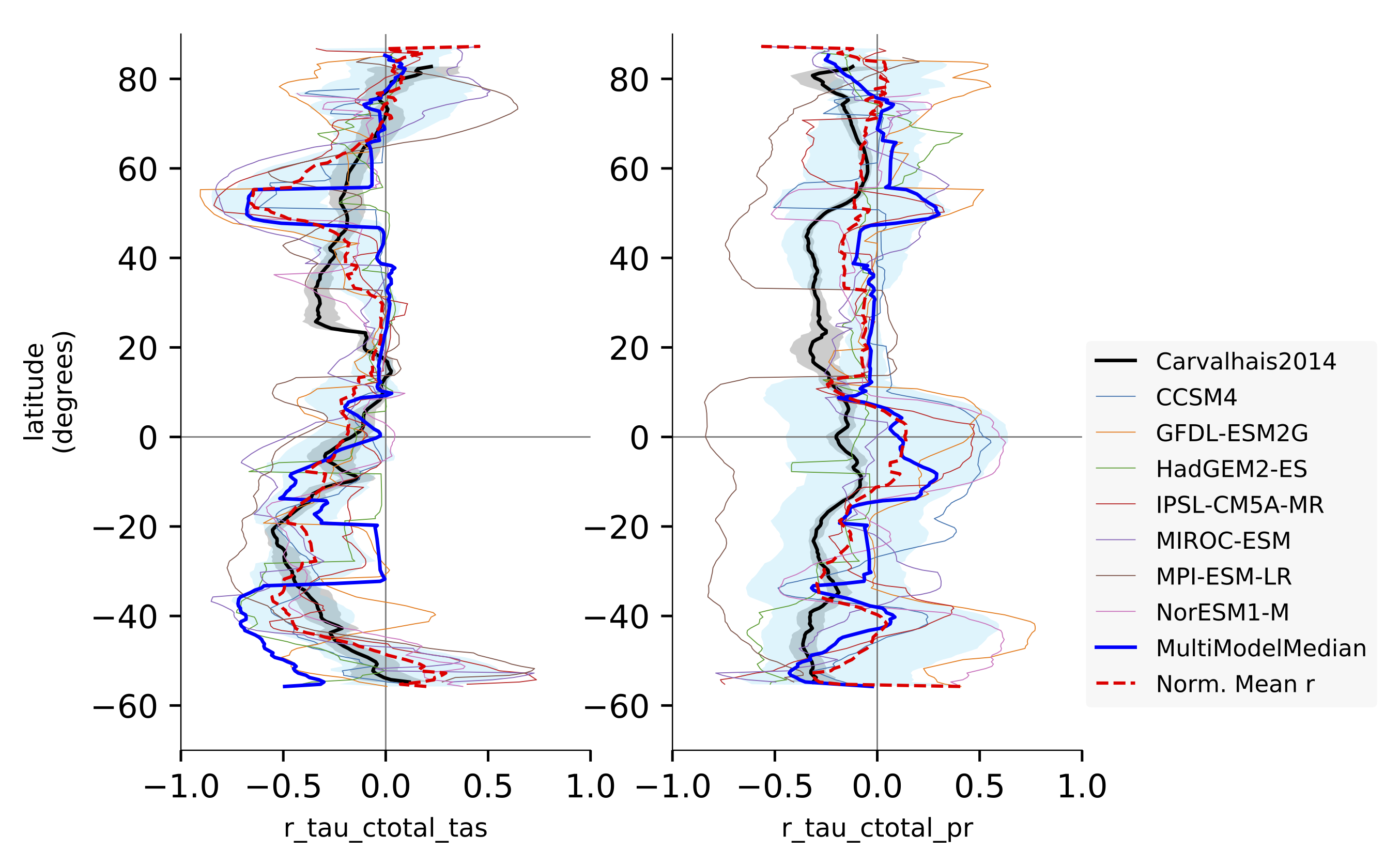
_images/r_tau_ctotal_climate_pearson_Carvalhais2014_gnz.png — Fig. 18 Comparison of latitudinal (zonal) variations of pearson correlation between turnover time and climat…#

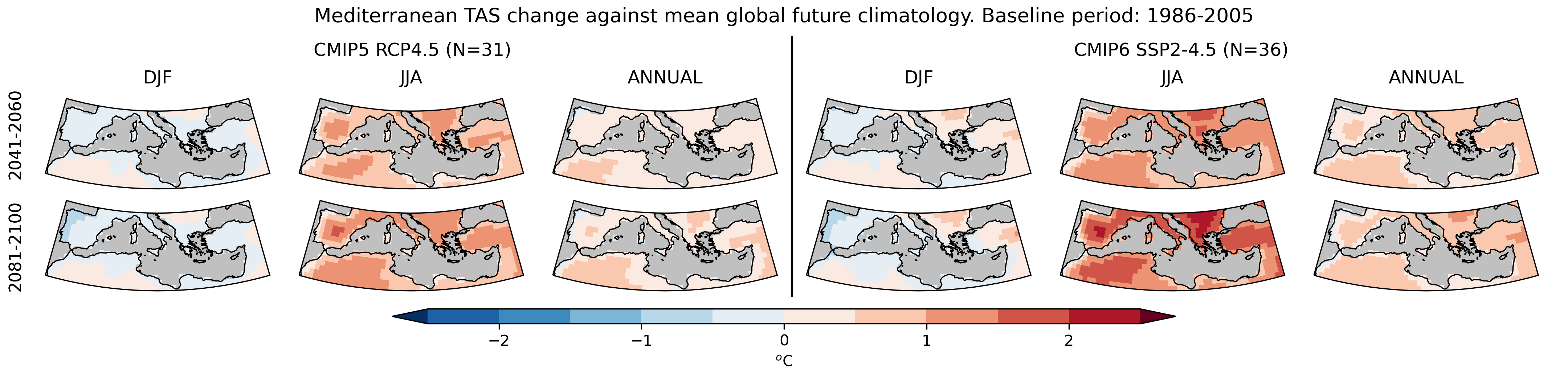
_images/tas_45.png — Fig. 19 Mediterranean region temperature change differences against the mean global temperature change. The …#

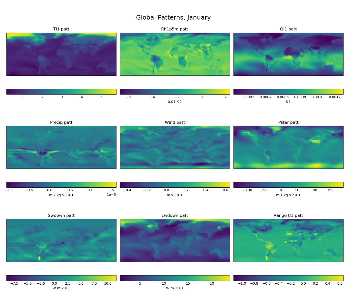
_images/patterns.png — Fig. 20 Patterns generated for CMIP6 models, gridded view. Patterns are shown per variable, for the month of…#

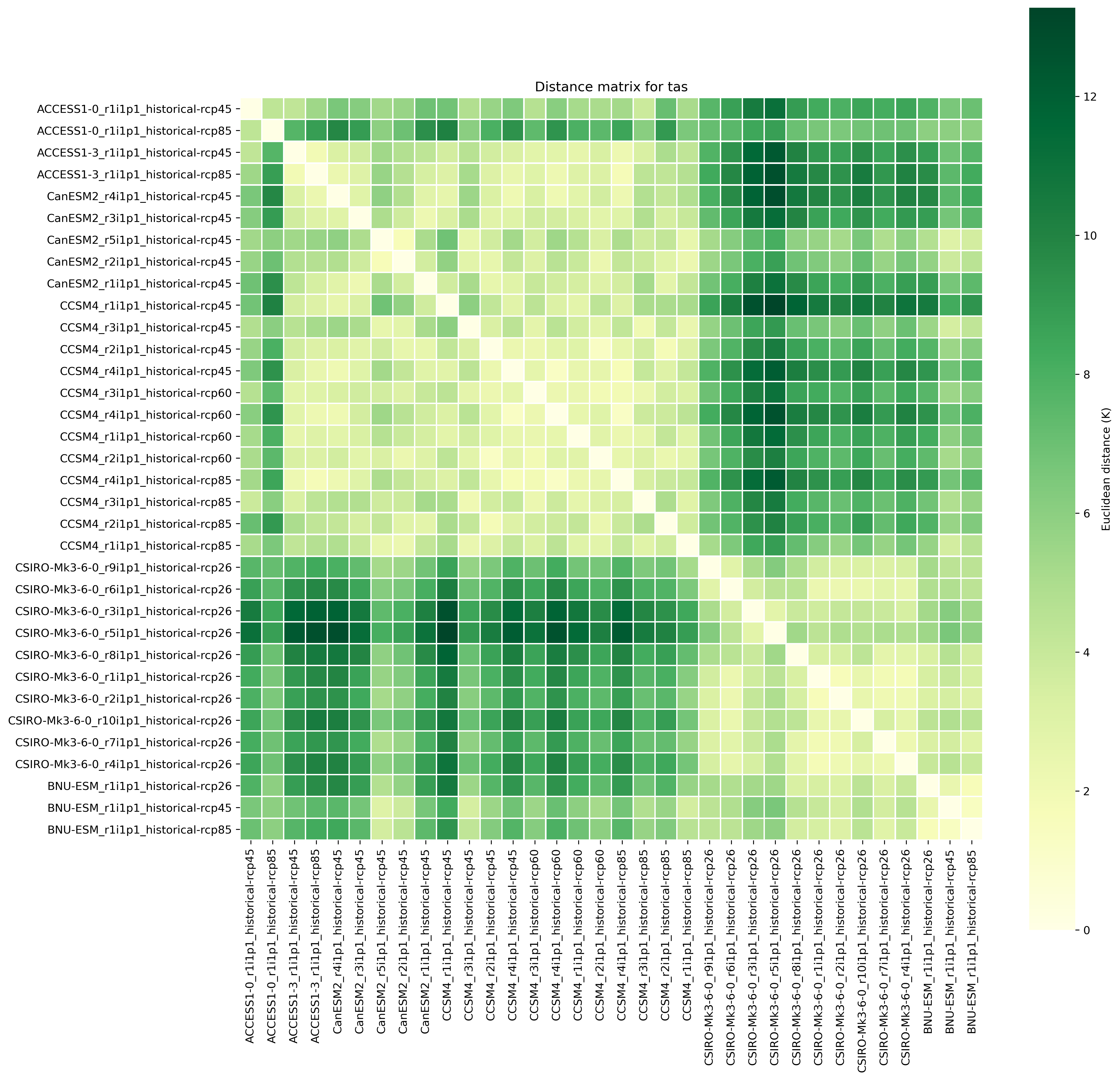
_images/independence_tas.png — Fig. 21 Distance matrix for temperature, providing the independence metric.#

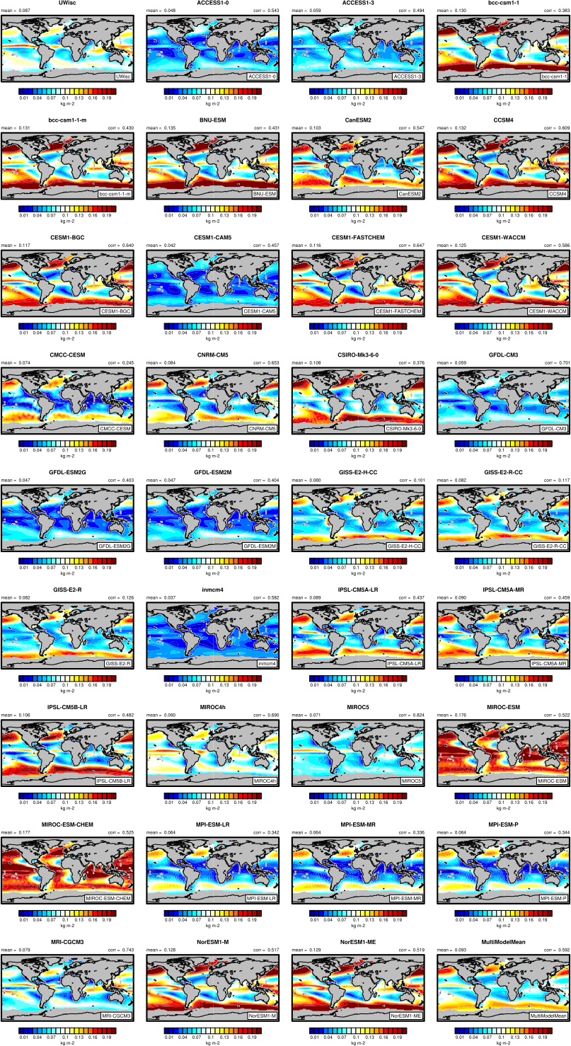
_images/clouds_lwp_annual.png — Fig. 22 The 20-yr average LWP (1986-2005) from the CMIP5 historical model runs and the multi-model mean in c…#

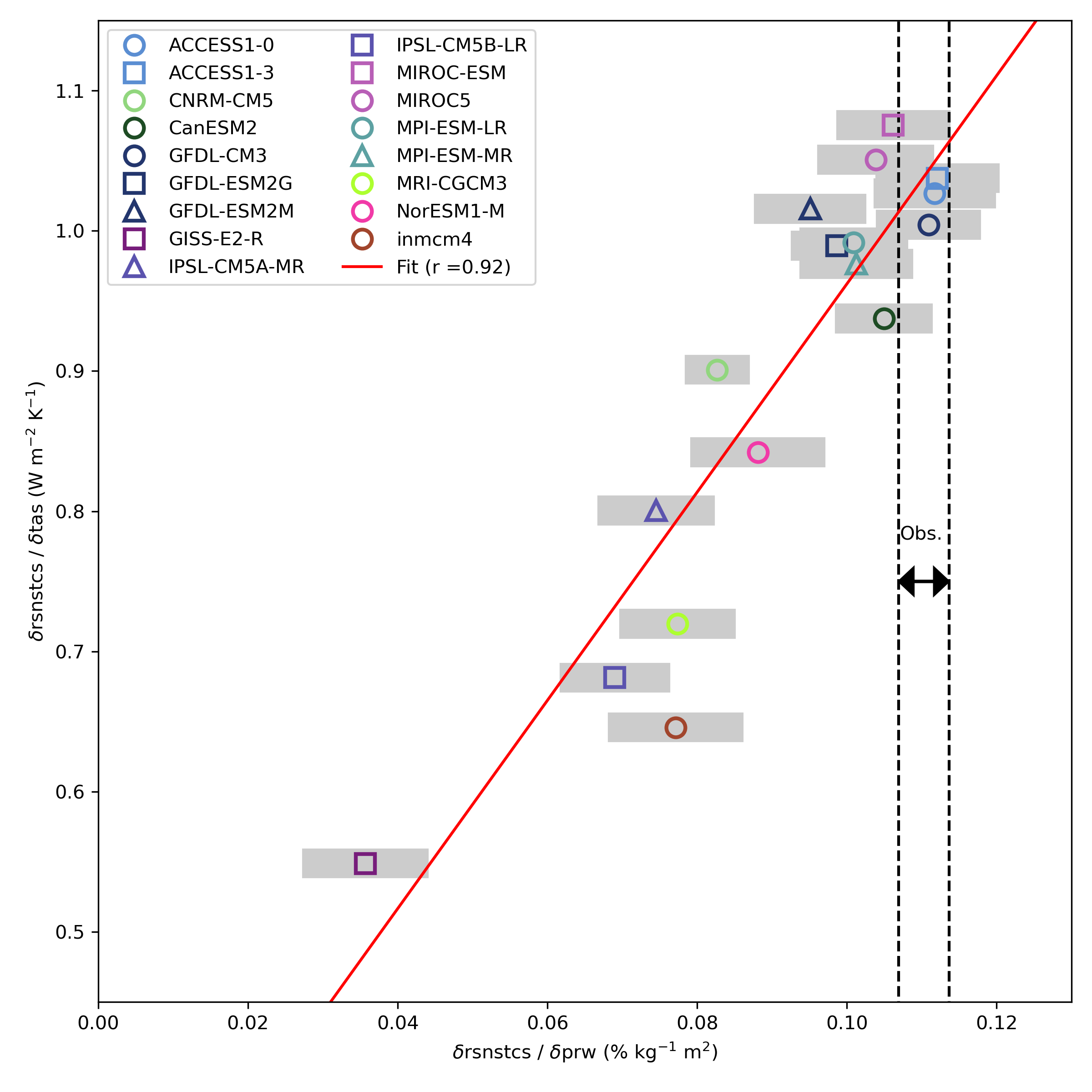
_images/fig_deangelis_cmug_cdr2.png — Fig. 23 Scatter plot and regression line computed between the ratio of the change of net short wave radiatio…#

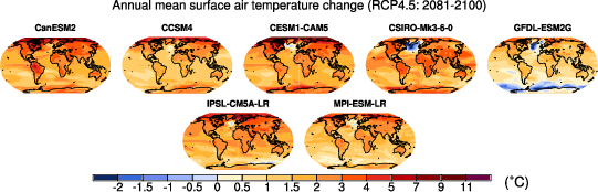
_images/collins_fig_1.png — Fig. 24 Surface air temperature change in 2081–2100 displayed as anomalies with respect to 1986–2005 for RCP…#

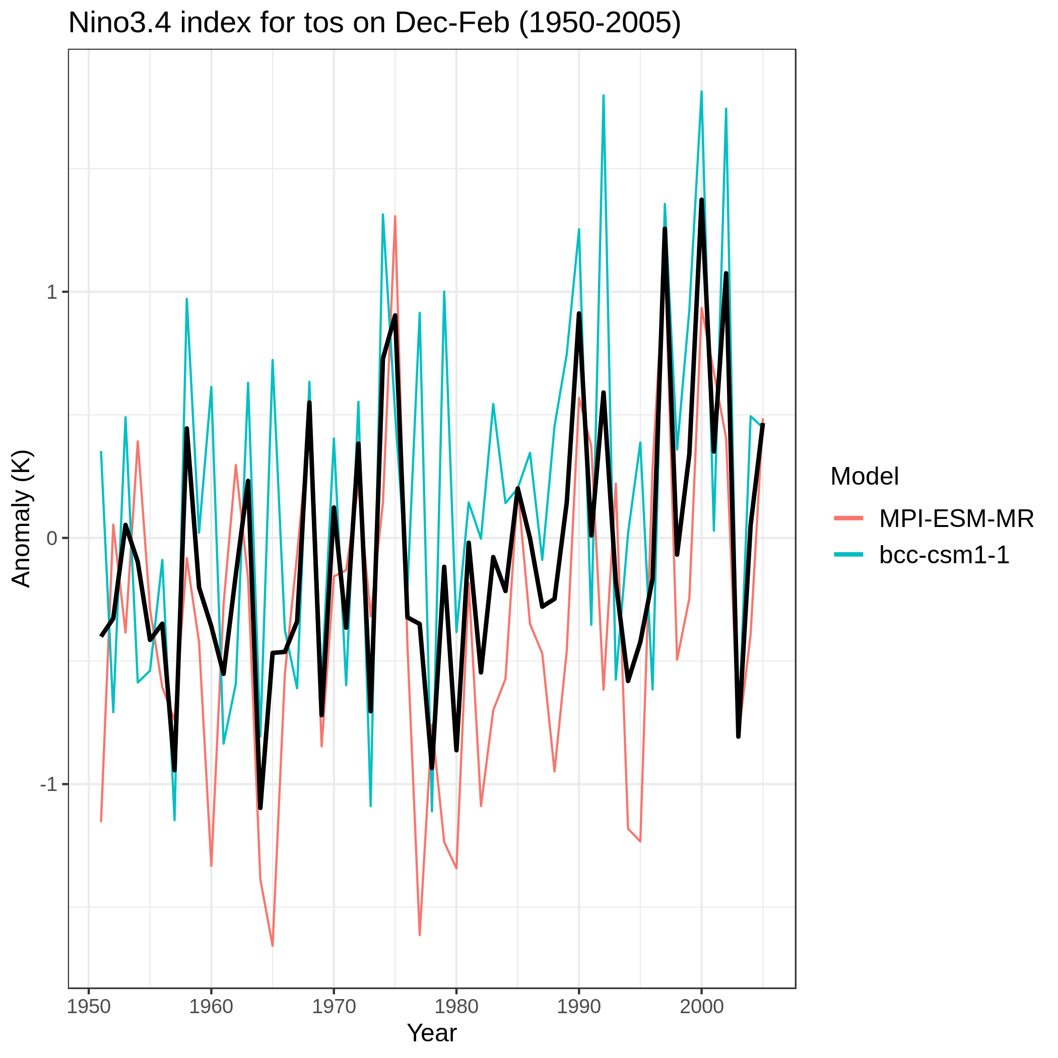
_images/Nino3.4_tos_Dec-Feb_running-mean__1950-2005.png — Fig. 25 Time series of the standardized sea surface temperature (tos) area averaged over the Nino 3.4 region…#

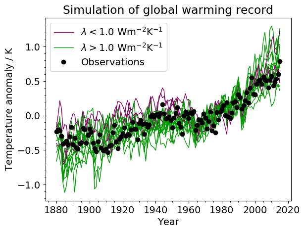
_images/temperature_anomaly_HadCRUT4.png — Fig. 26 Simulated change in global temperature from CMIP5 models (coloured lines), compared to the global te…#

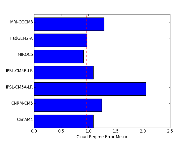
_images/crem_error_metric.png — Fig. 27 Cloud Regime Error Metrics (CREMpd) from William and Webb (2009) applied to selected CMIP5 AMIP simu…#

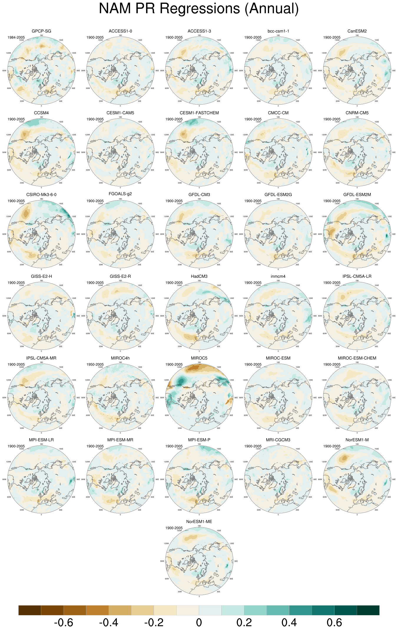
_images/nam.prreg.ann.png — Fig. 28 Regression of the precipitation anomalies (PR) onto the Northern Annular Mode (NAM) index for the ti…#

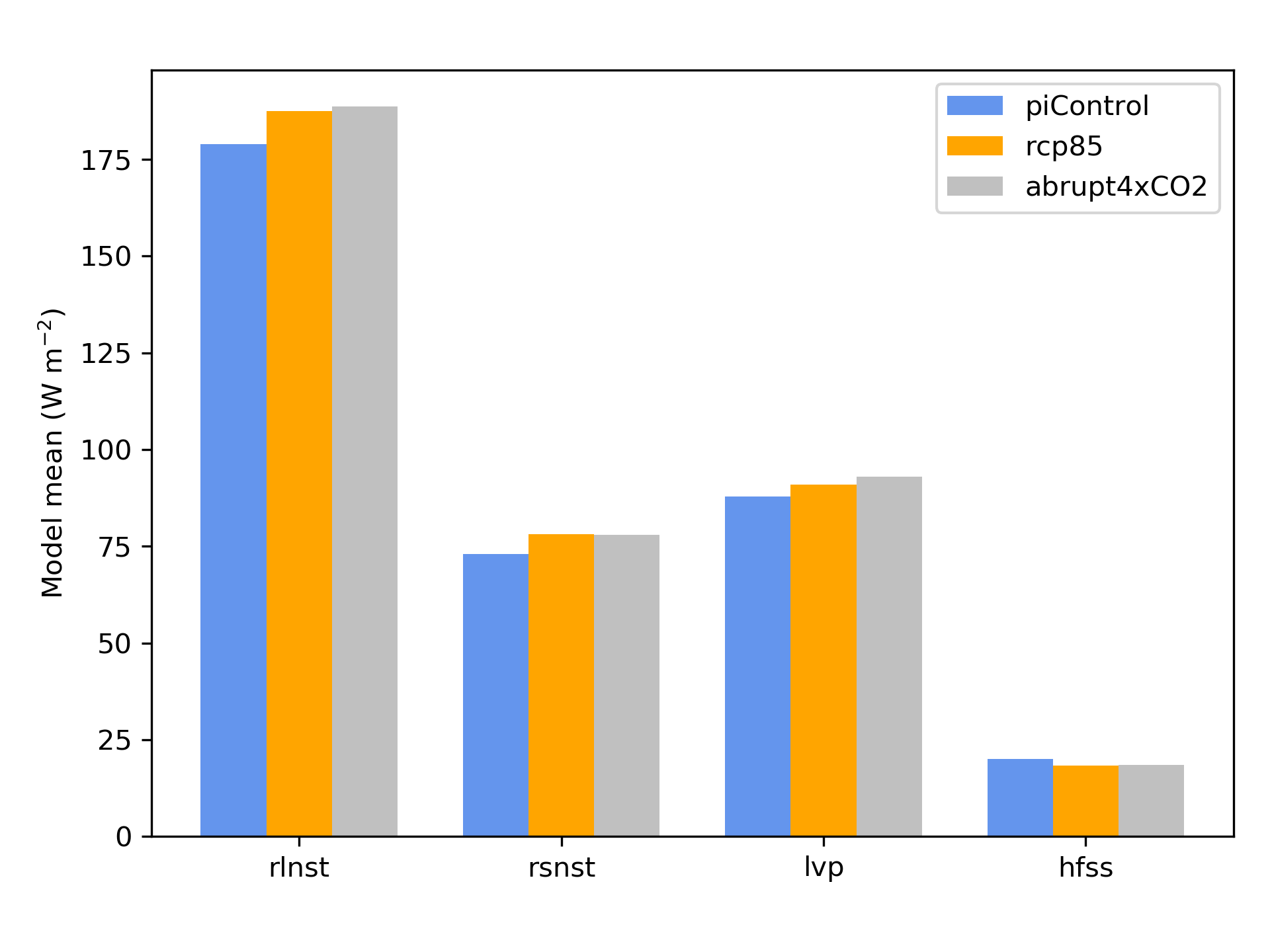
_images/bar_all.png — Fig. 29 Global average multi-model mean comparing different model experiments for the sum of upward long wav…#

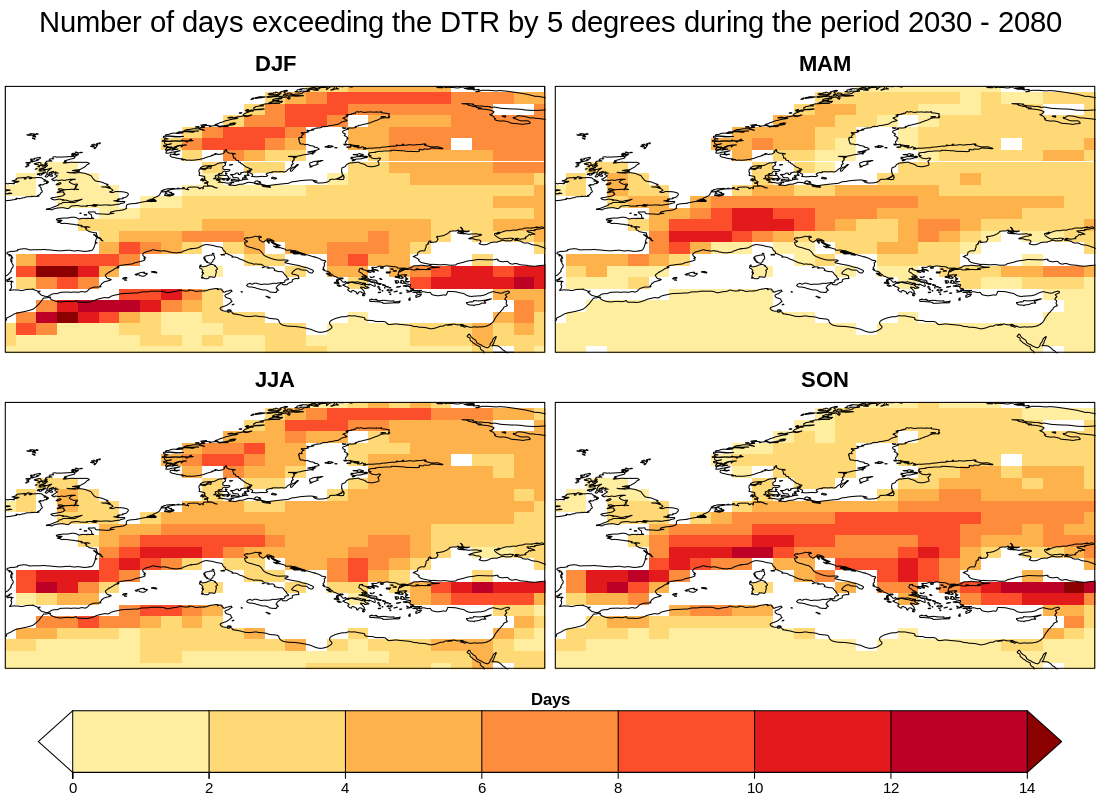
_images/Seasonal_DTRindicator_MPI-ESM-MR_2030_2080_1961_1990.png — Fig. 30 Mean number of days exceeding the Diurnal Temperature Range (DTR) simulated during the historical pe…#

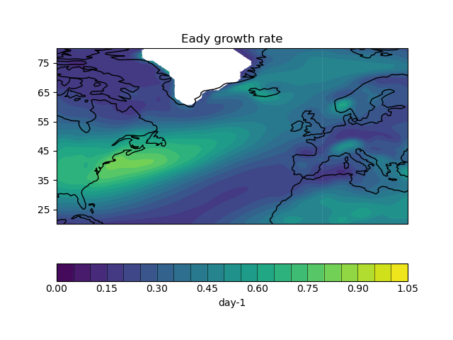
_images/HadGEM3-GC31-LM_winter_eady_growth_rate_70000.png — Fig. 31 Eady Growth Rate values over the North-Atlantic region at 70000 Pa.#

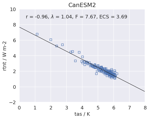
_images/CanESM2.png — Fig. 32 Scatterplot between TOA radiance and global mean surface temperature anomaly for 150 years of the ab…#

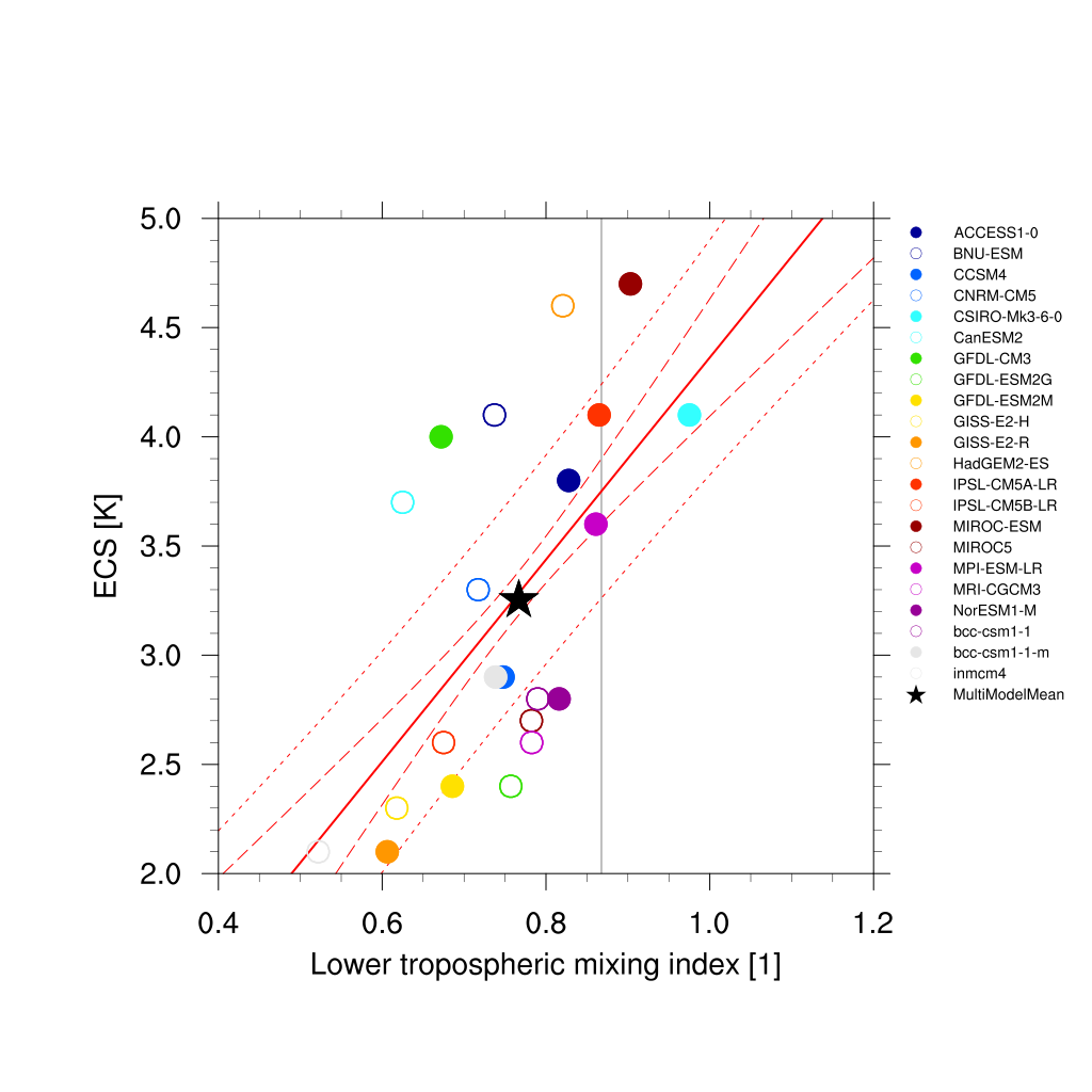
_images/ltmi.png — Fig. 33 Lower tropospheric mixing index (LTMI; Sherwood et al., 2014) vs. equilibrium climate sensitivity fr…#

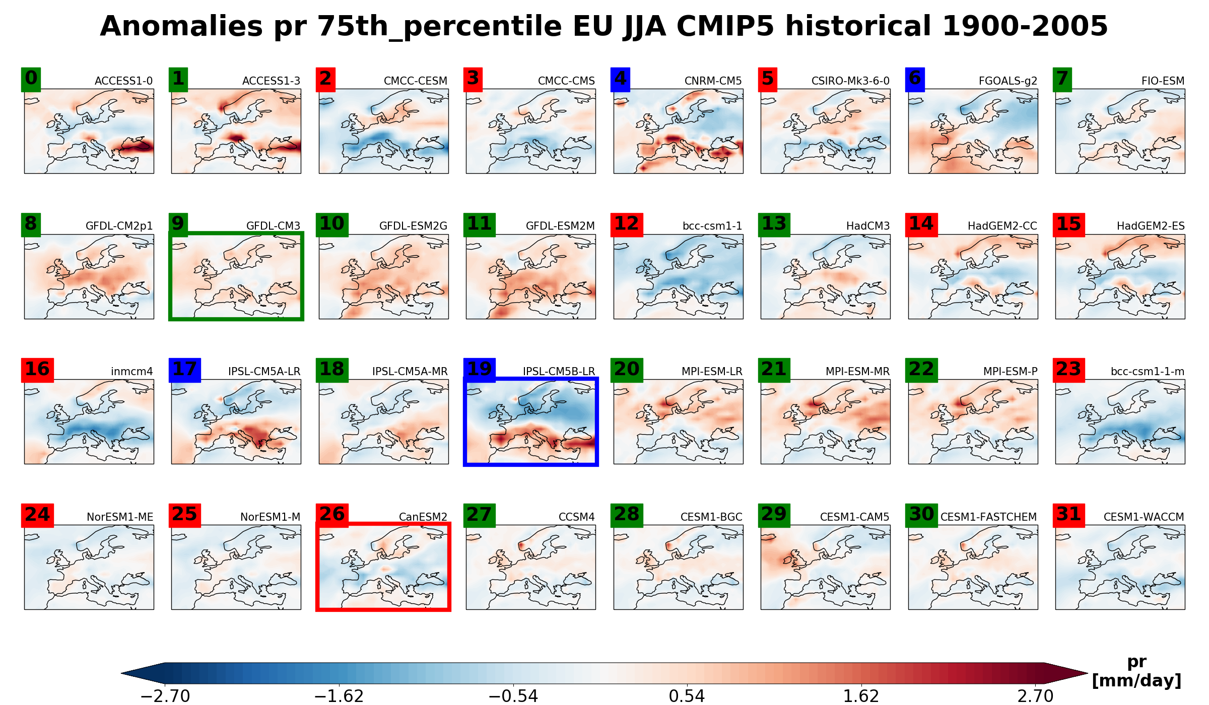
_images/ensclus.png — Fig. 34 Clustering based on the 75th percentile of historical summer (JJA) precipitation rate for CMIP5 mode…#

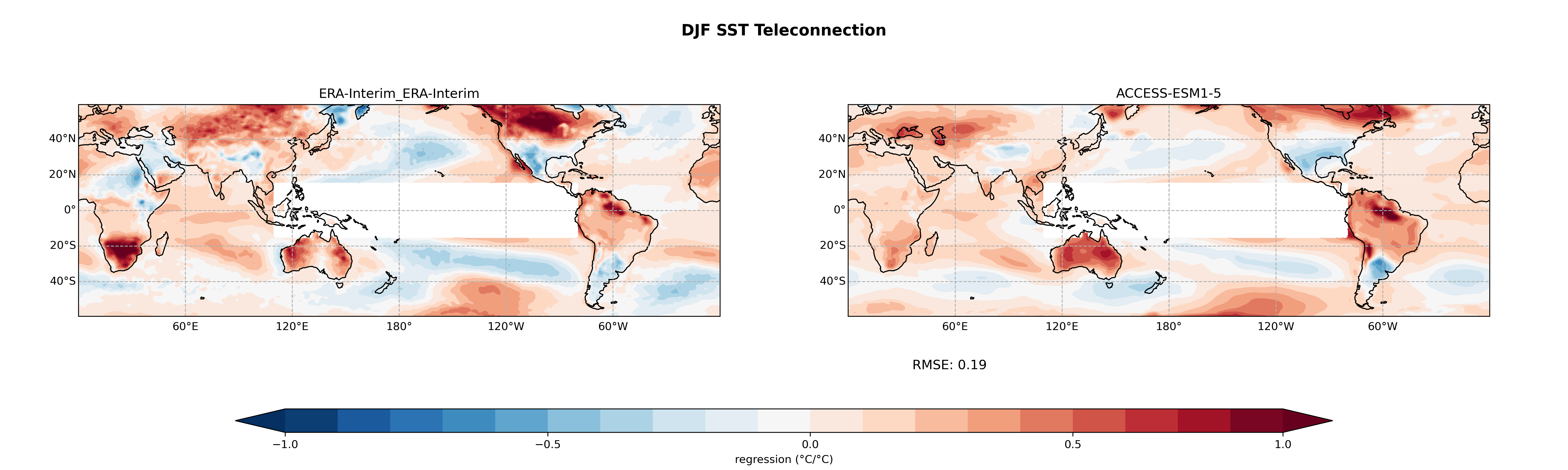
_images/ACCESS-ESM1-5_DJF_ts_telecon.png — Fig. 35 PR or SST anomalies on Earth (between 60°S-60°N), showing the location associated with ENSO.#

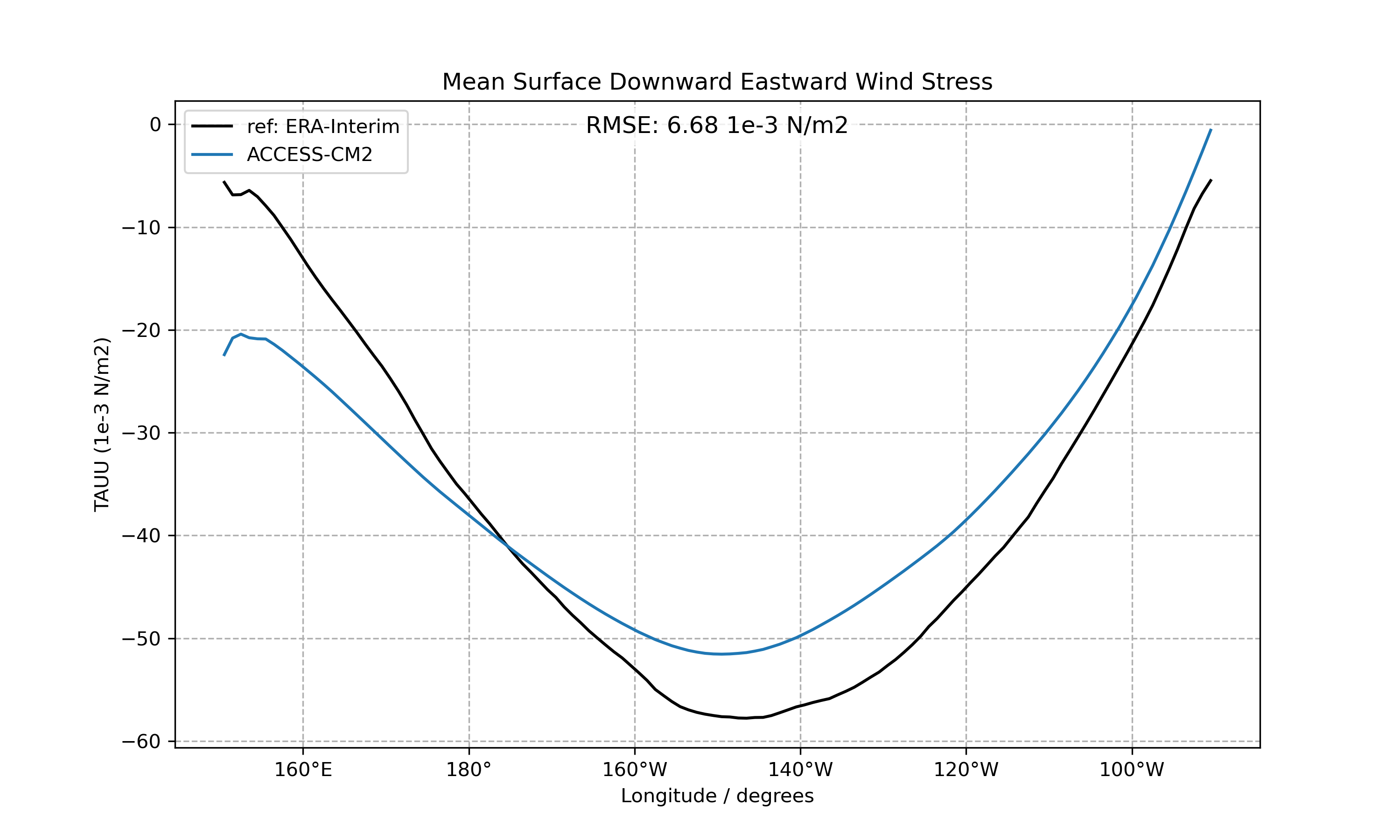
_images/ACCESS-CM2_eq_tauu_bias.png — Fig. 36 Bias in the zonal structure of zonal wind stress (Taux) in the equatorial Pacific (5°S-5°N averaged)…#

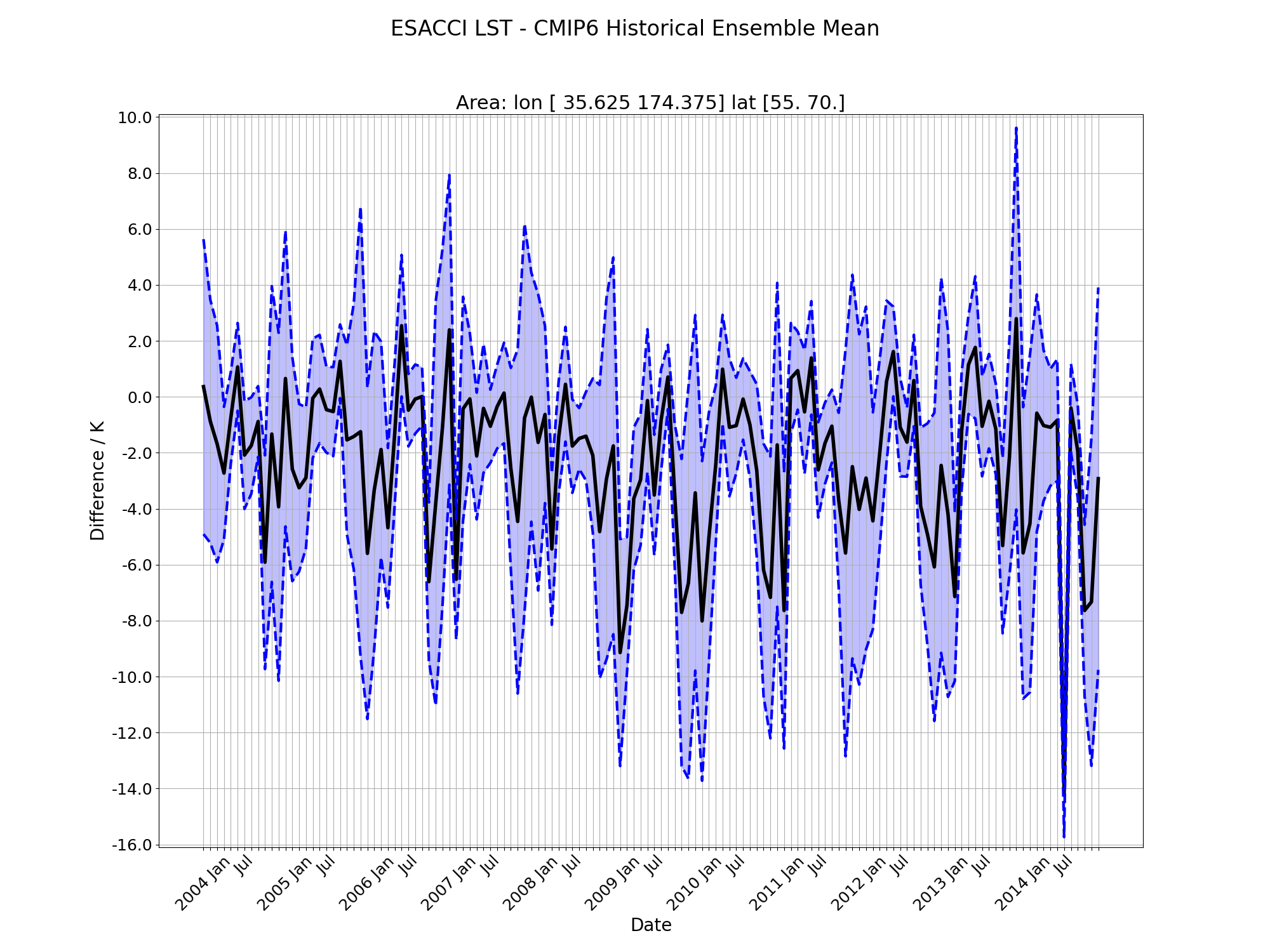
_images/lst_example.png — Fig. 37 Timeseries of the ESA CCI LST minus mean of CMIP6 ensembles. The selected region is 35E-175E, 55N-70…#

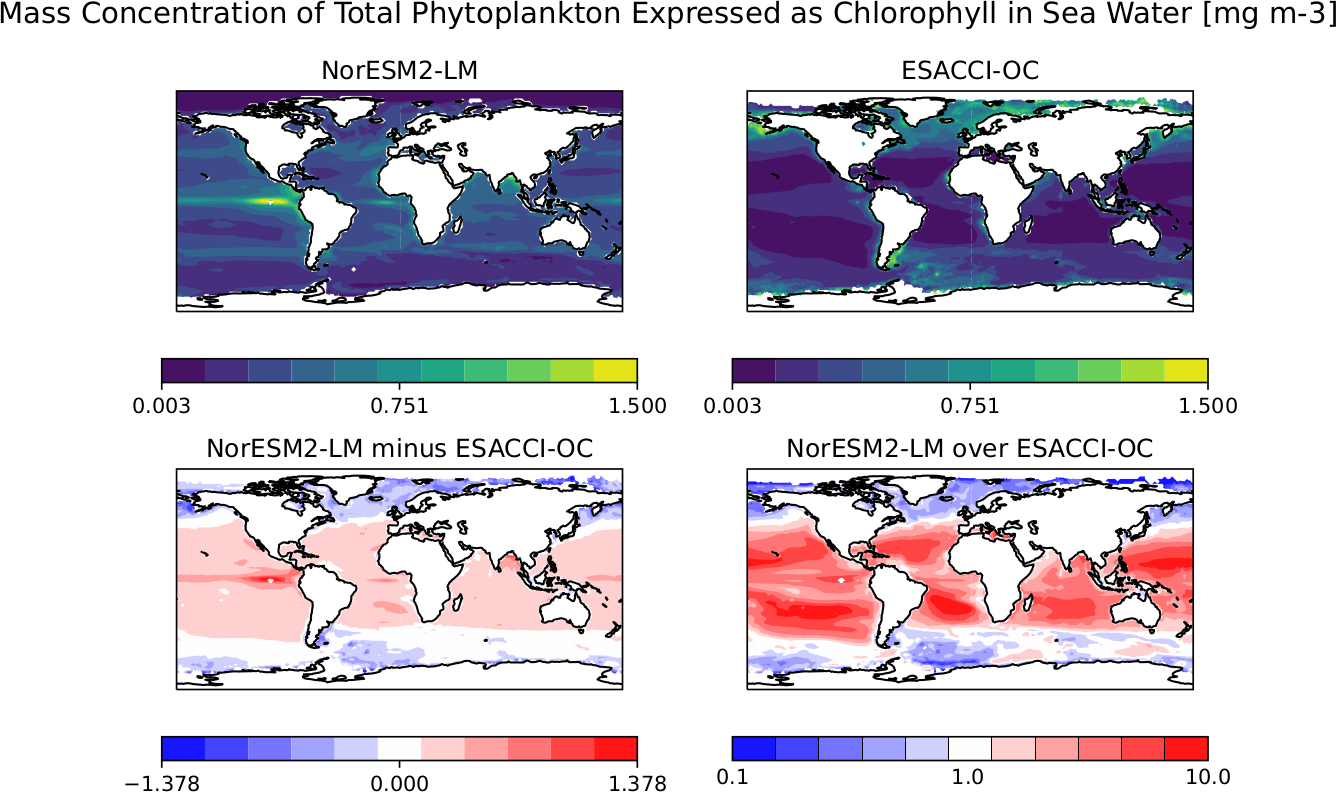
_images/model_vs_obs_MassConcentrationofTotalPhytoplanktonExpressedasChlorophyllinSeaWater_NorESM2-LM_ESACCI-OC__maps.png — Fig. 38 Surface chlorophyll from ESACCI-OC ocean colour data version 5.0 and the CMIP6 model NorESM2-LM. Thi…#

_images/map.png — Fig. 39 Air temperature in January 2000 (BCC-ESM1 CMIP6).#

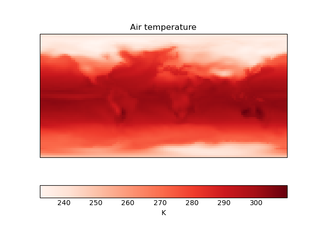
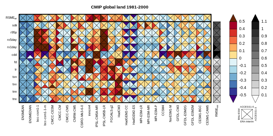
_images/gleckler.png — Fig. 40 Portrait plot of relative error metrics for the CMIP5 temperature and precipitation extreme indices …#

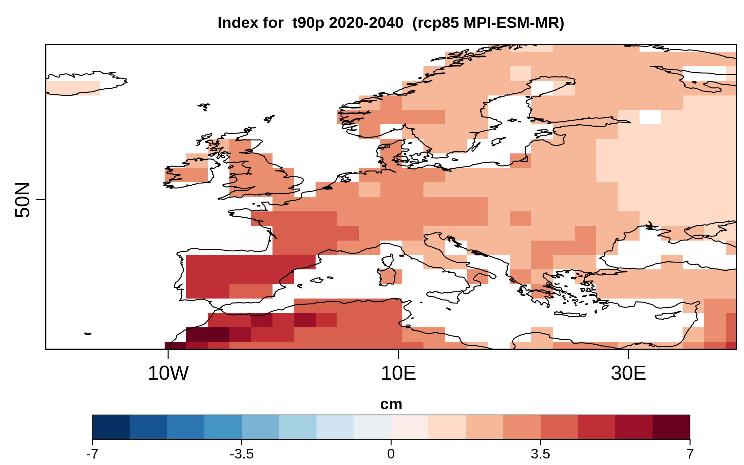
_images/t90p_IPSL-CM5A-LR_rcp85_2020_2040.png — Fig. 41 Average change in the heat component (t90p metric) of the Combined Climate Extreme Index for the 202…#

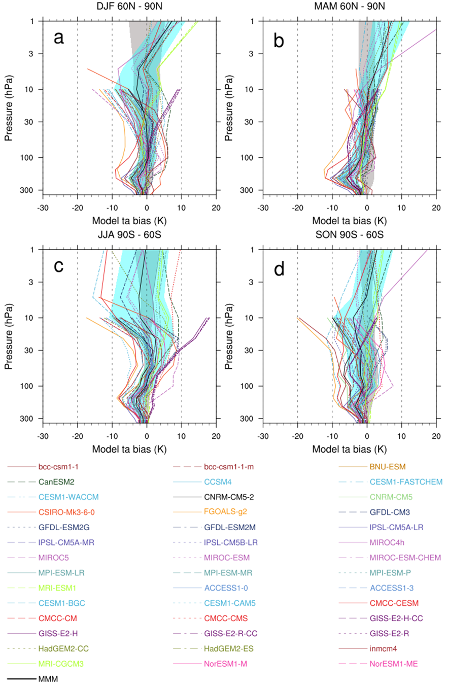
_images/fig_diagn01.png — Fig. 42 Climatological mean temperature biases for (top) 60–90N and (bottom) 60–90S for the (left) winter an…#

_images/fig_eyr13jgr_12.png — Fig. 43 Long-term mean (thin black contour) and linear trend (colour) of zonal mean DJF zonal winds for the …#

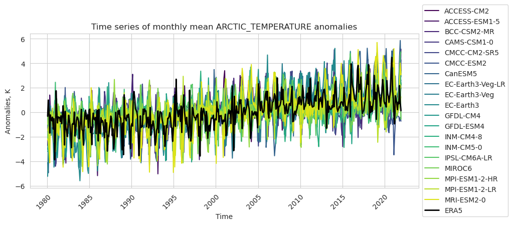
_images/Timeseries_Arctic_temperature_anomalies.png — Fig. 44 Monthly mean temperature anomalies in the Arctic (65°–90°N) from observations and selected CMIP6 mod…#

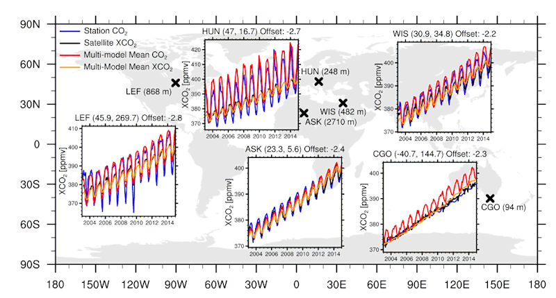
_images/fig02.png — Fig. 45 Comparison of time series from satellite, in situ, and models sampled accordingly. Caveat: inset plo…#

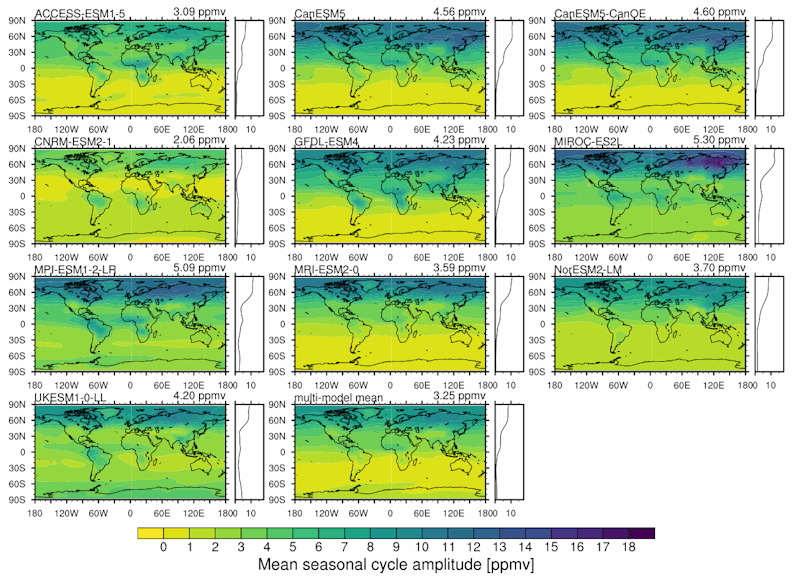
_images/fig05.png — Fig. 46 Panel plot of spatially resolved seasonal cycle amplitude for all models, including a zonal average …#

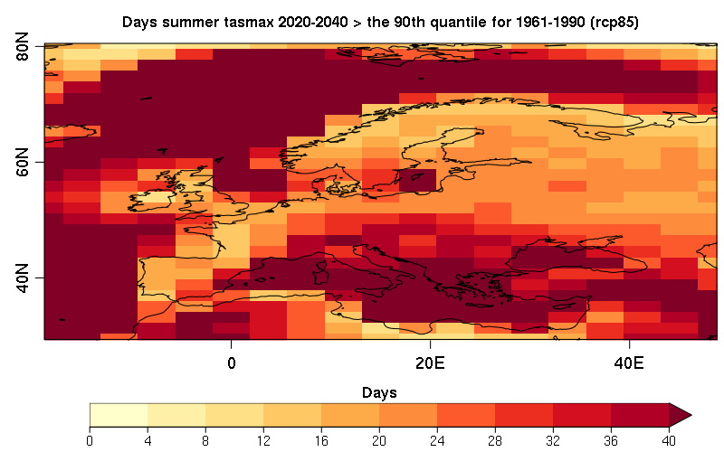
_images/tasmax_extreme_spell_durationsummer_IPSL-CM5A-LR_rcp85_2020_2040.png — Fig. 47 Mean number of summer days during the period 2060-2080 when the daily maximum near-surface air tempe…#

_images/Precipitation_day_plot.png — Fig. 48 Precipitation per day for 2015-01-01:2016-12-31.#

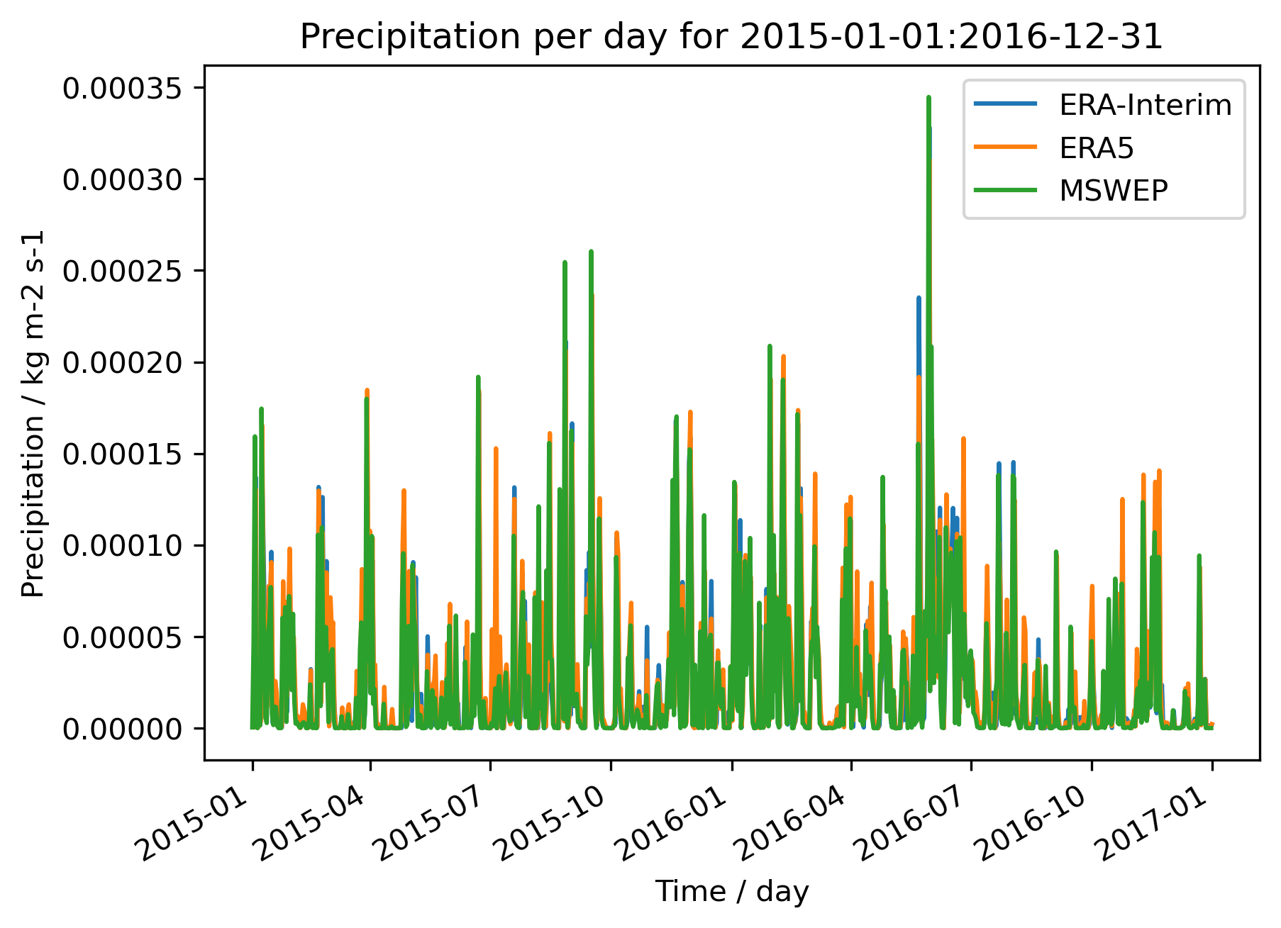
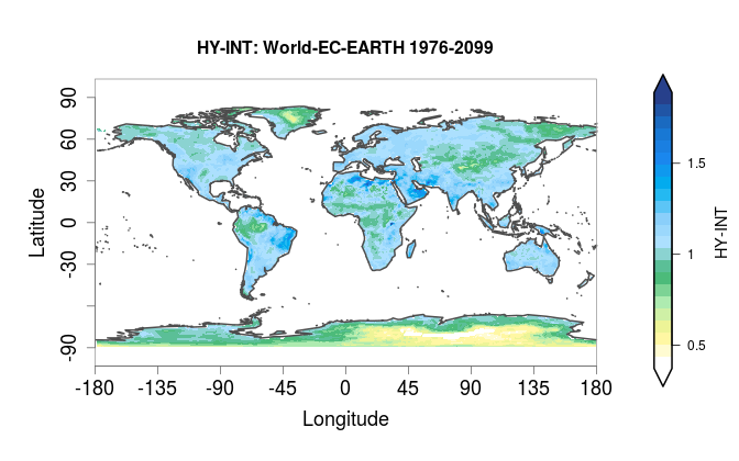
_images/hyint_maps.png — Fig. 49 Mean hydroclimatic intensity for the EC-EARTH model, for the historical + RCP8.5 projection in the p…#

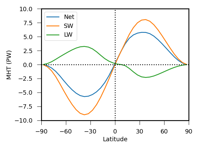
_images/figure1_CERES-EBAF_CERES-EBAF.png — Fig. 50 The implied heat transport due to the total net flux (blue), split into the contributions from the S…#

_images/bias_vs_change.png — Fig. 51 Bias and change for each variable#

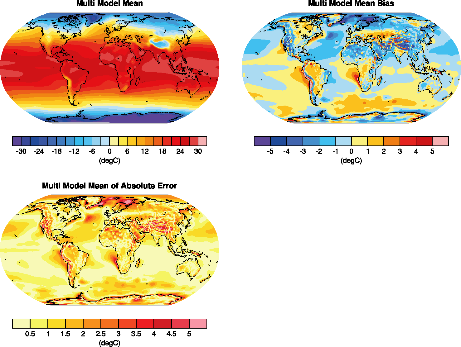
_images/fig-9-2.png — Fig. 52 Figure 9.2 a,b,c: Annual-mean surface air temperature for the period 1980-2005. a) multi-model mean,…#

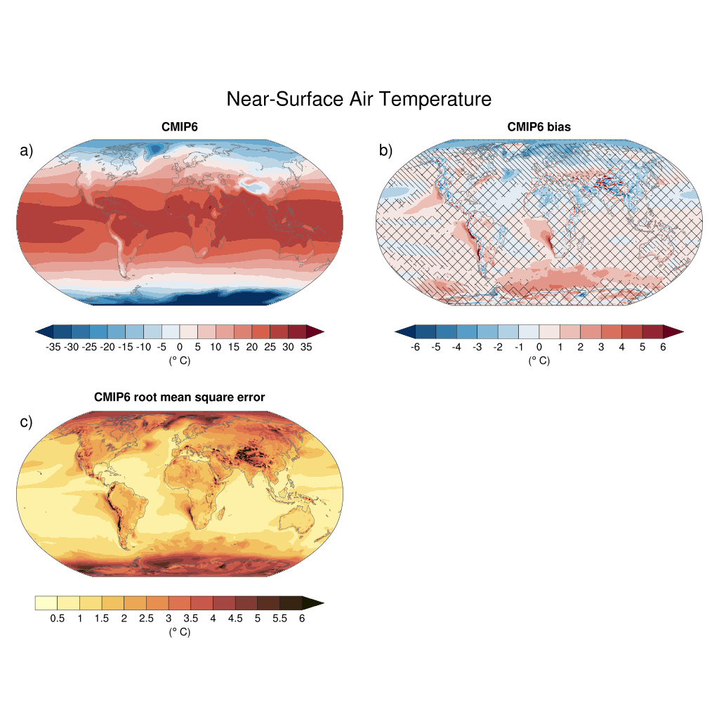
_images/model_bias_tas_annualclim_CMIP6.png — Fig. 53 Figure 3.3: Annual mean near-surface (2 m) air temperature (°C) for the period 1995-2014. (a) Multi-…#

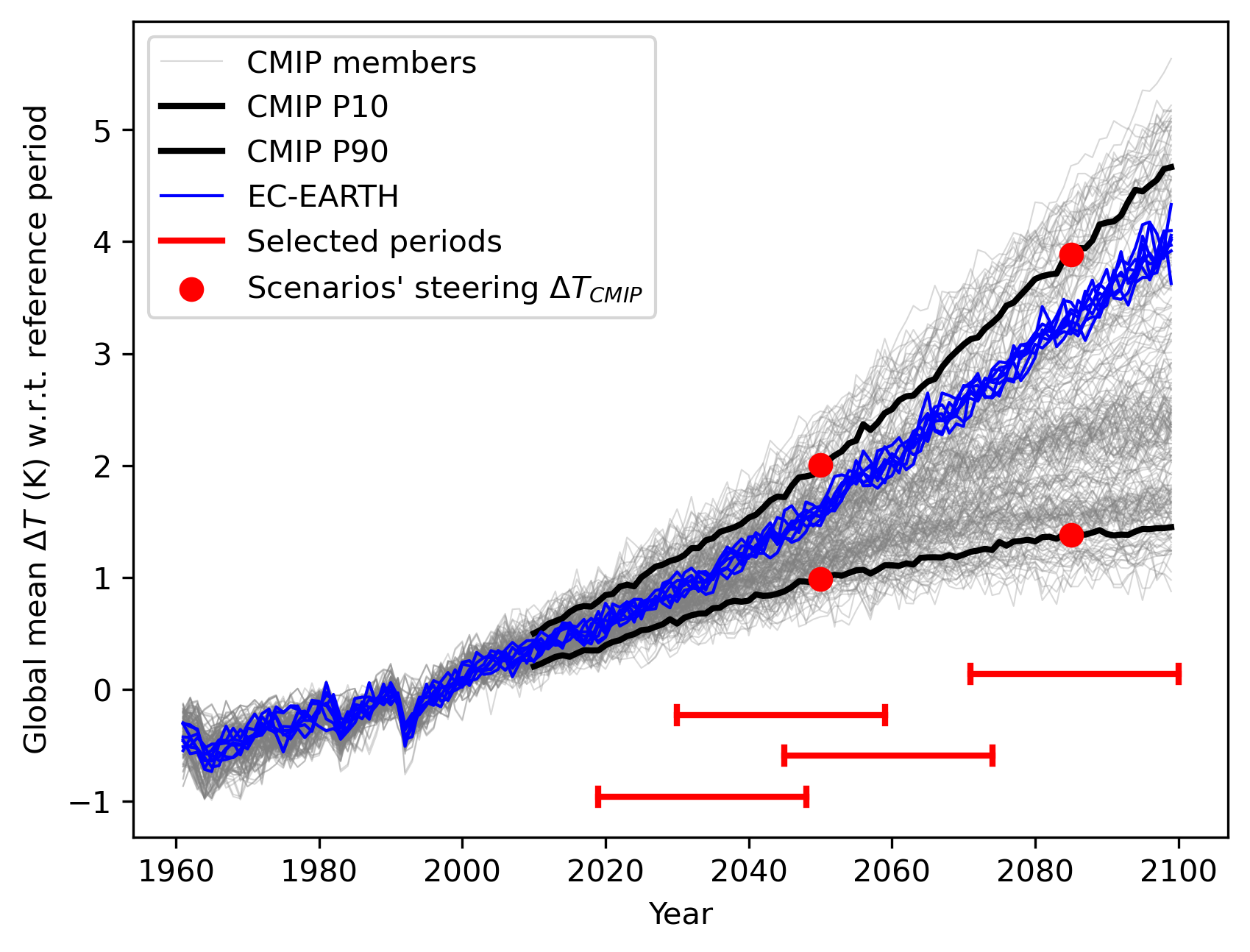
_images/global_matching.png — Fig. 54 CMIP spread in global temperature change, highlighting selected steering parameters and resampling p…#

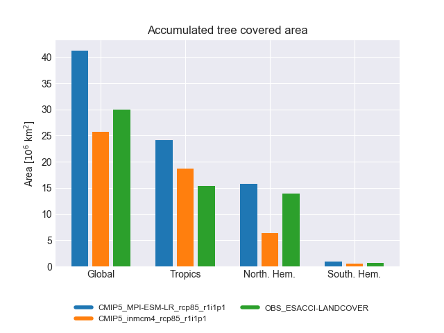
_images/area_treeFrac.png — Fig. 55 Accumulated tree covered area for different regions and experiments.#

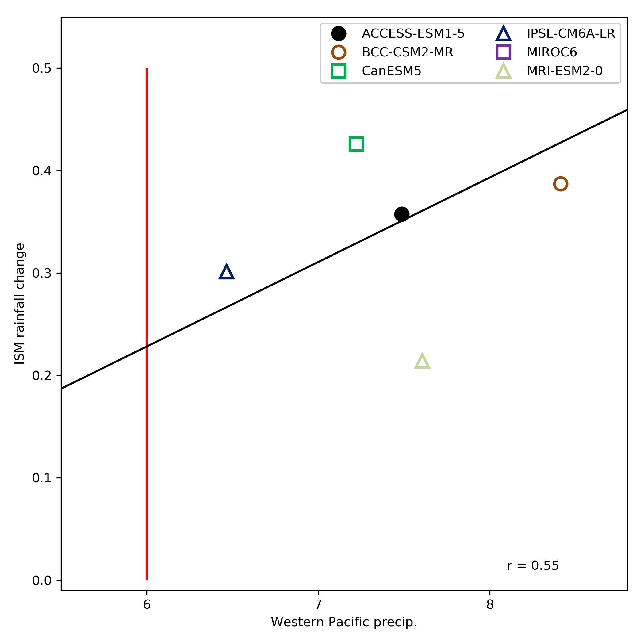
_images/li17natcc_fig2a.png — Fig. 56 Scatter plot of the simulated tropical western Pacific precipitation (mm d-1) versus projected avera…#

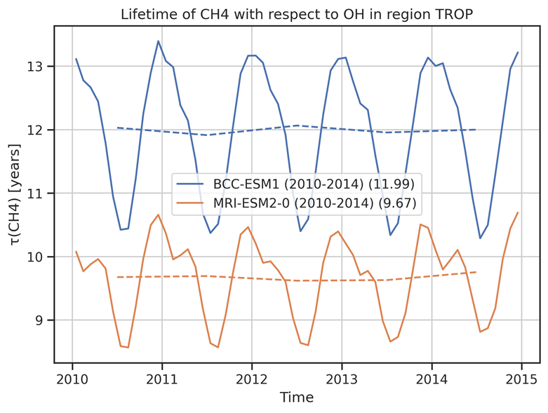
_images/timeseries_ambiguous_dataset_ch4_TROP.png — Fig. 57 No caption available#

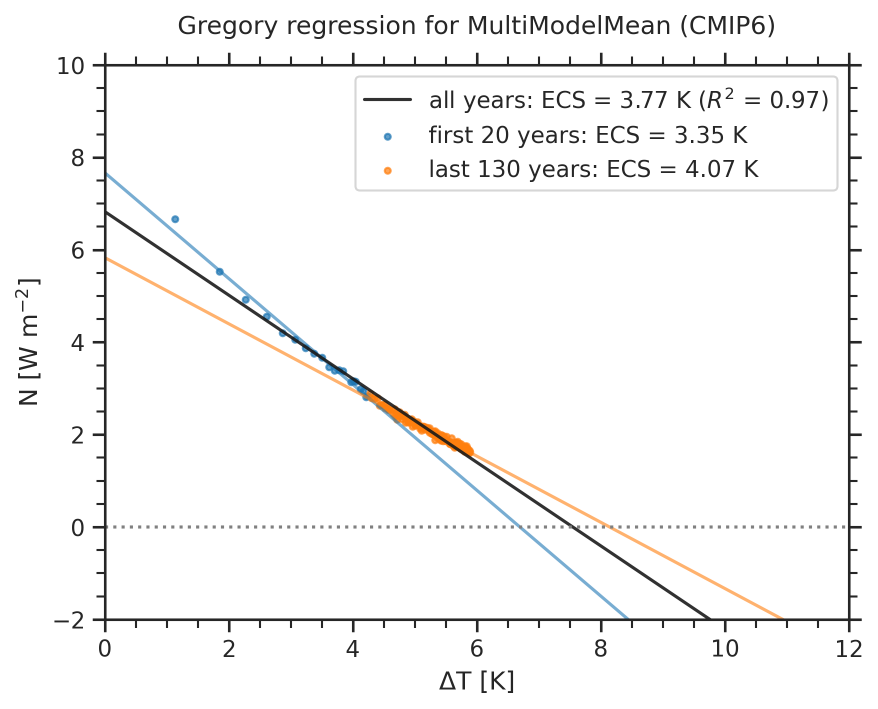
_images/cmip6_gregory_regression.png — Fig. 58 ECS calculated for the CMIP6 models using the Gregory method over different time scales. Using the e…#

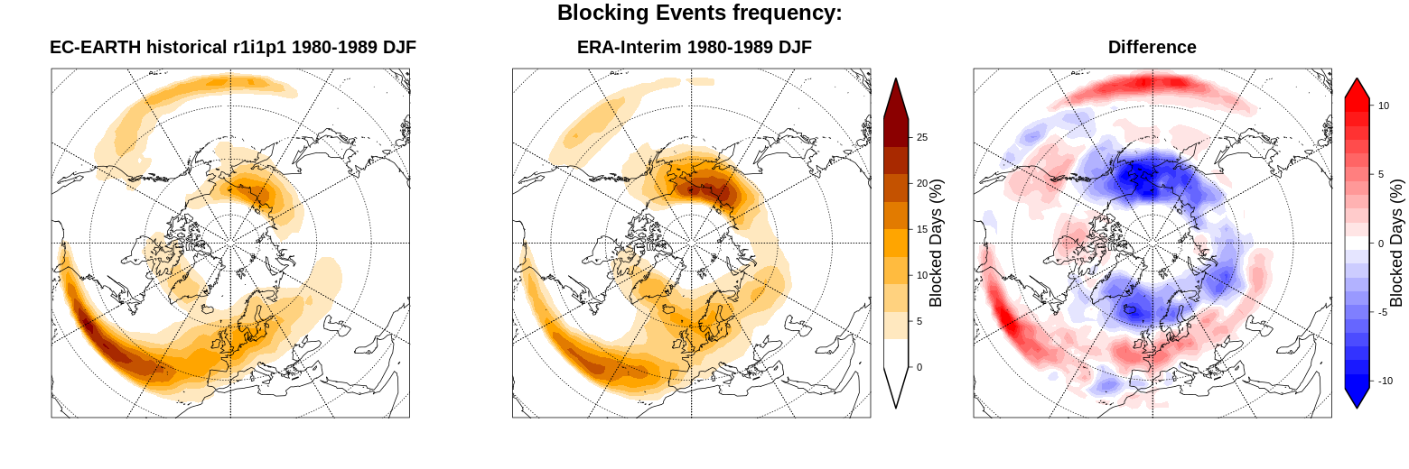
_images/miles_block.png — Fig. 59 Blocking Events frequency for a CMIP5 EC-Earth historical run (DJF 1980-1989), compared to ERA-Inter…#

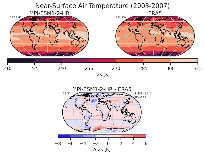
_images/map_tas_MPI-ESM1-2-HR_Amon.jpg — Fig. 60 Global climatology of 2m near-surface air temperature.#

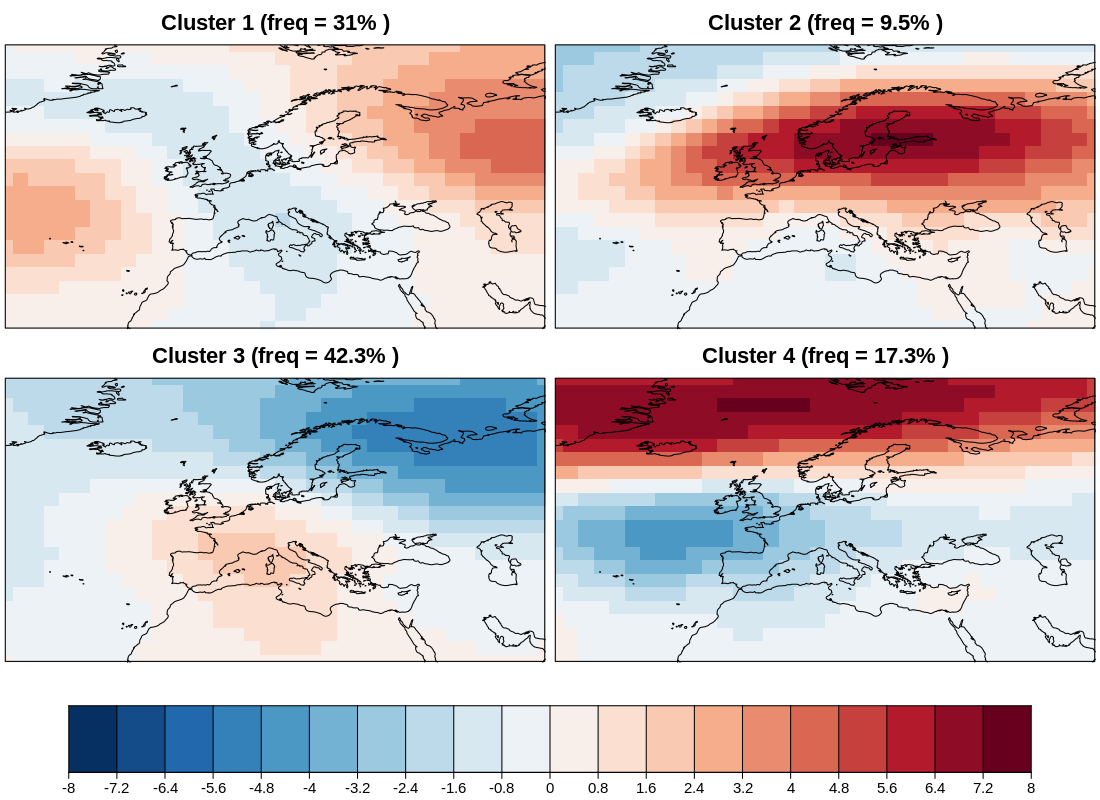
_images/SON-psl_predicted_regimes.png — Fig. 61 Four modes of variability for autumn (September-October-November) in the North Atlantic European Sec…#

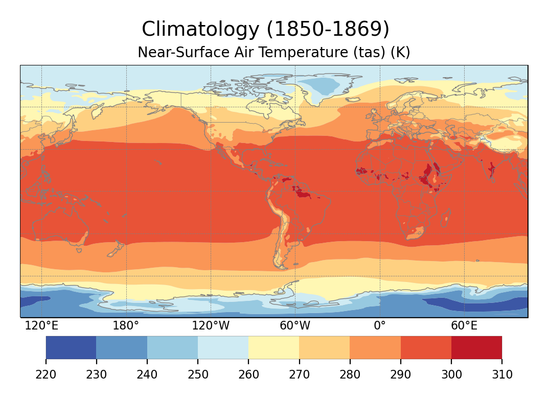
_images/clim.png — Fig. 62 Global climatology of tas.#

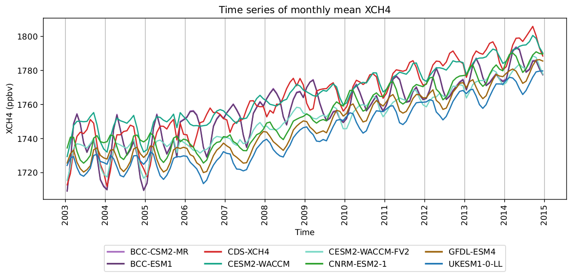
_images/lineplot_xch4_2003-2014_monmean.png — Fig. 63 Monthly mean time series of XCH4, calculated over the whole globe, for individual CMIP6 model simula…#

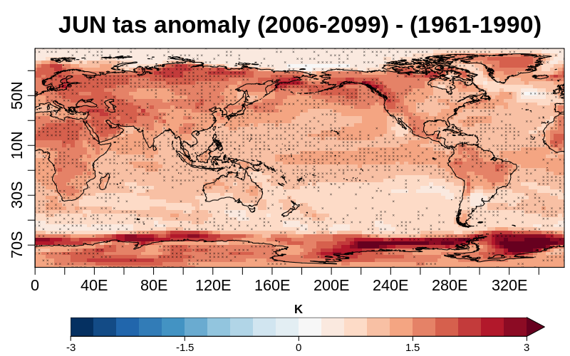
_images/tas_JUN_multimodel-anomaly_2006_2099_1961_1990.png — Fig. 64 Multi-model mean anomaly of 2-m air temperature during the future projection 2006-2099 in June consi…#

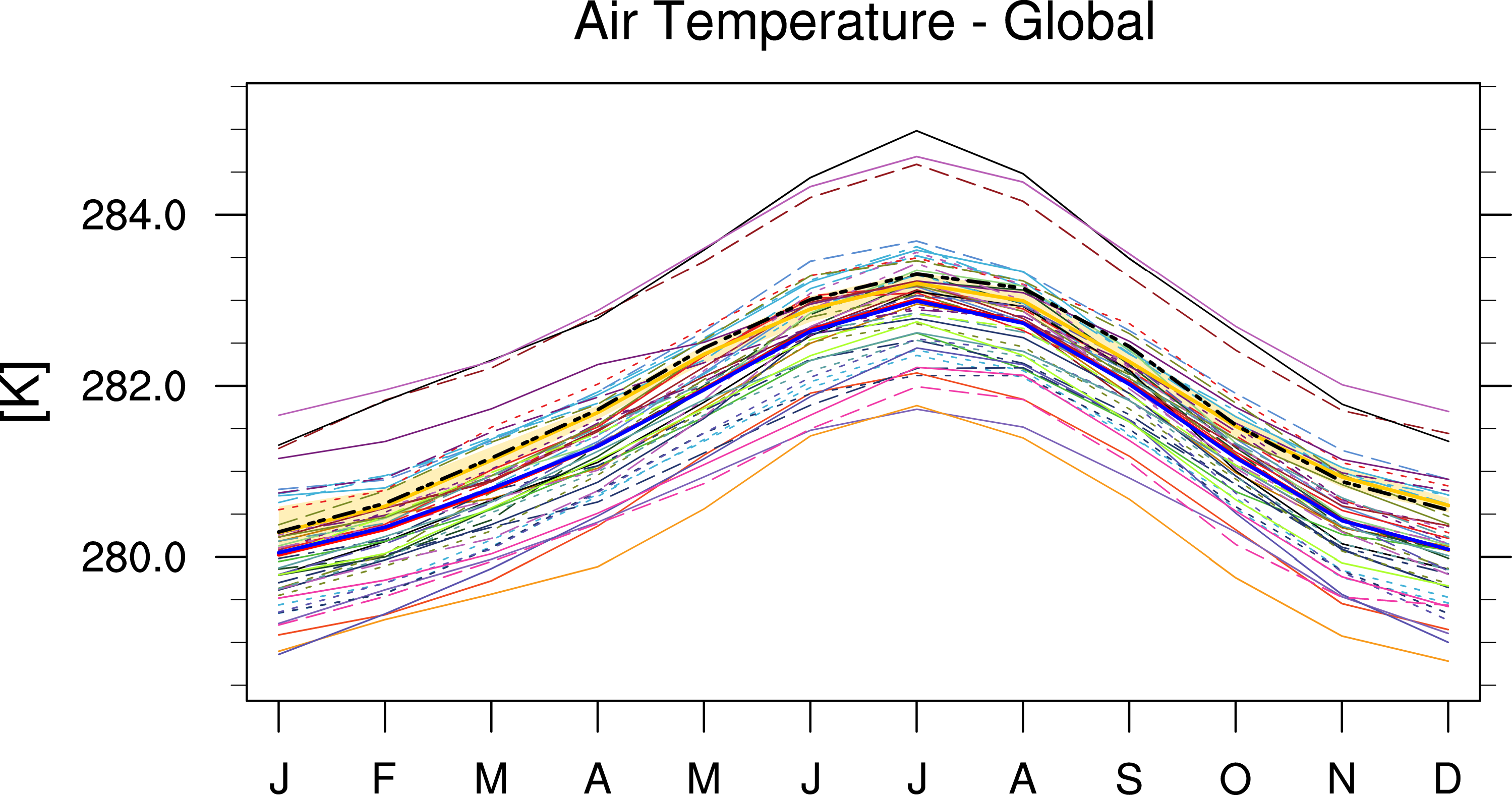
_images/perfmetrics_fig_1.png — Fig. 65 Annual cycle of globally averaged temperature at 850 hPa (time period 1980-2005) for different CMIP5…#

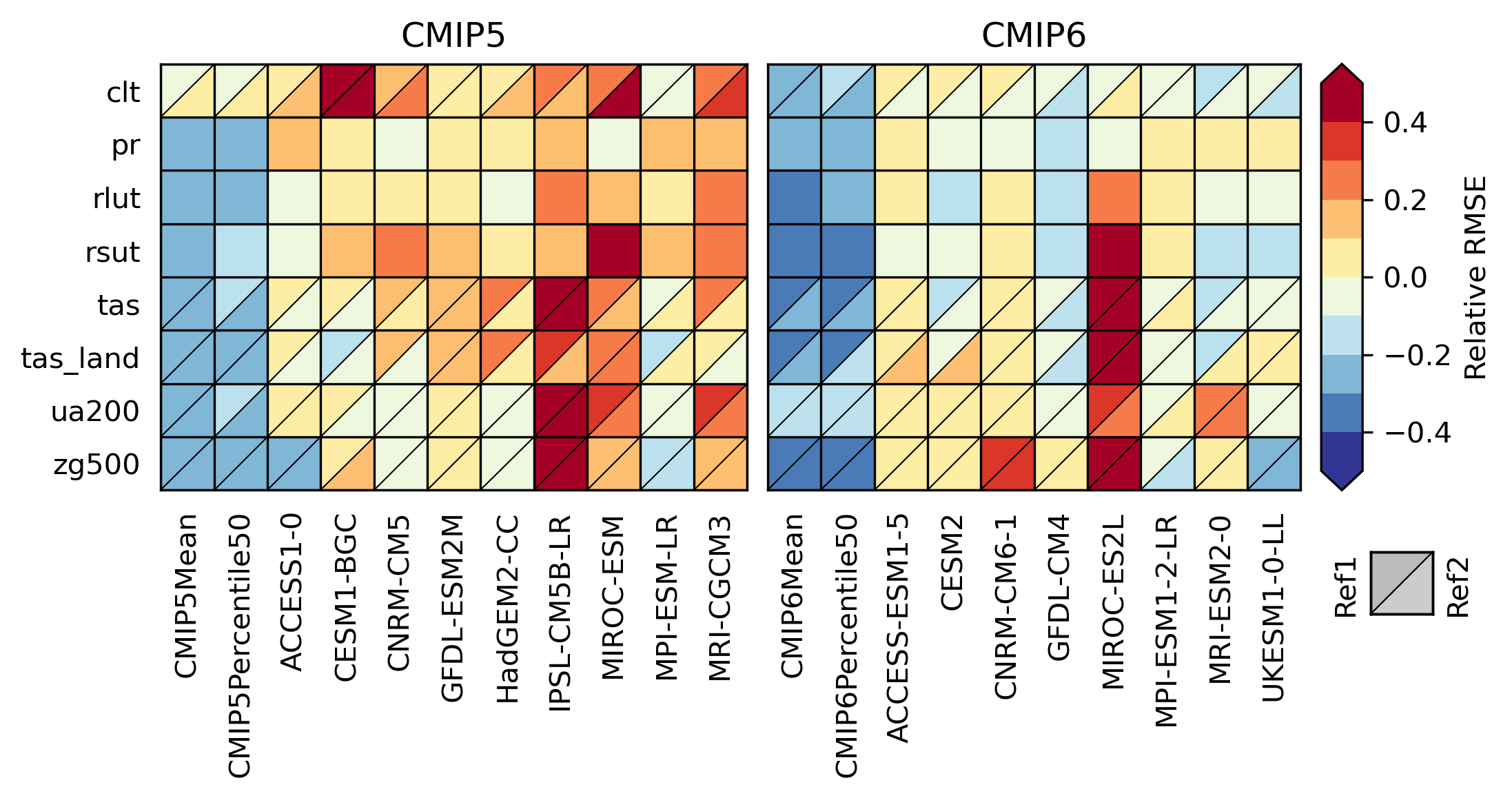
_images/portrait_plot.png — Fig. 66 Relative space-time root-mean-square deviation (RMSD) calculated from the climatological seasonal cy…#

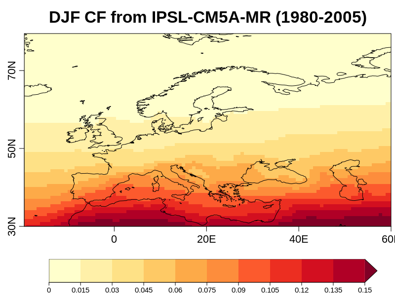
_images/capacity_factor_IPSL-CM5A-MR_1980-2005_DJF.png — Fig. 67 PV capacity factor calculated from IPSL-CM5-MR during the DJF season for 1980–2005.#

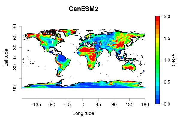
_images/quantilebias.png — Fig. 68 Quantile bias, as defined in Mehran et al. 2014, with threshold t=75th percentile, evaluated for the…#

_images/UKESM1-0-LL.png — Fig. 69 Radiation budget for UKESM1-0-LL#

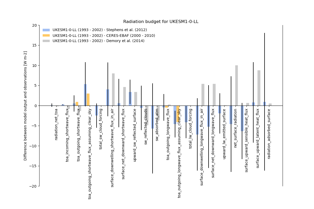
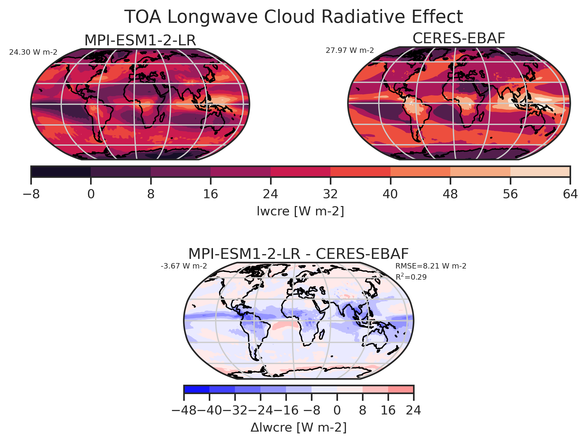
_images/map_lwcre_MPI-ESM1-2-LR_Amon.png — Fig. 70 Geographical map of the climatological mean longwave cloud radiative effect from MPI-ESM1-2-LR and C…#

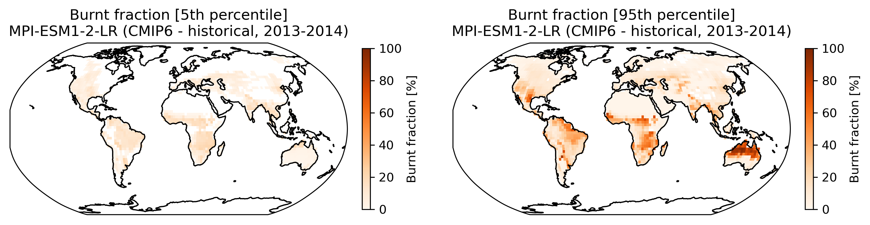
_images/burnt_fraction_MPI-ESM1-2-LR_historical_2013_2014.png — Fig. 71 Burnt area fraction for the MPI-ESM1-2-LR model (CMIP-historical experiment) for the time period 201…#

_images/catchments.png — Fig. 72 Catchment definitions used in the diagnostics.#

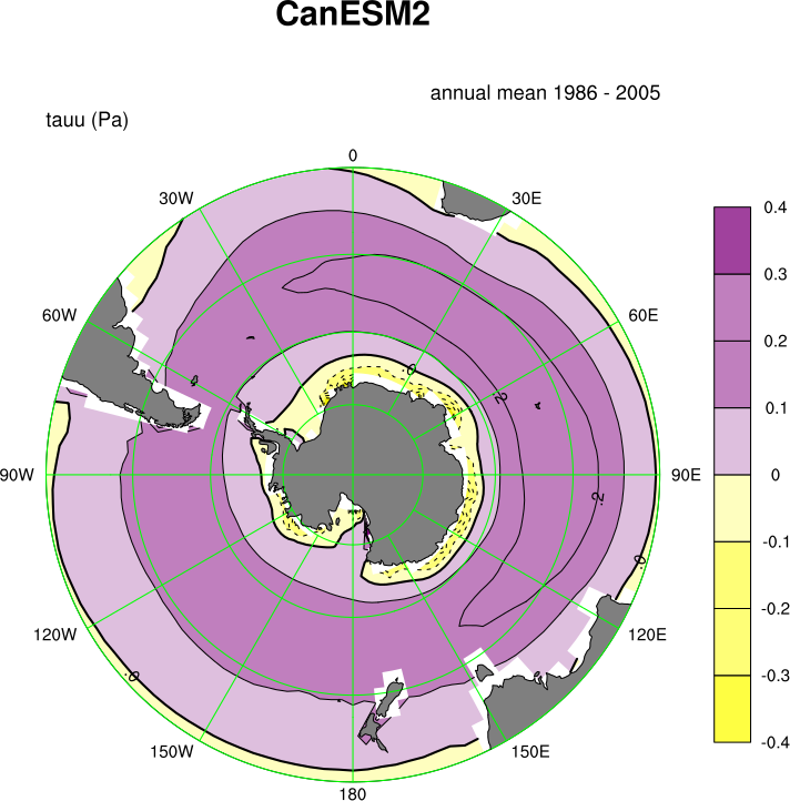
_images/Fig1_polar-contour_tauu_1986-2005.png — Fig. 73 Figure 1: Annual-mean zonal wind stress (tauu - N/m2) with eastward wind stress as positive plotted …#

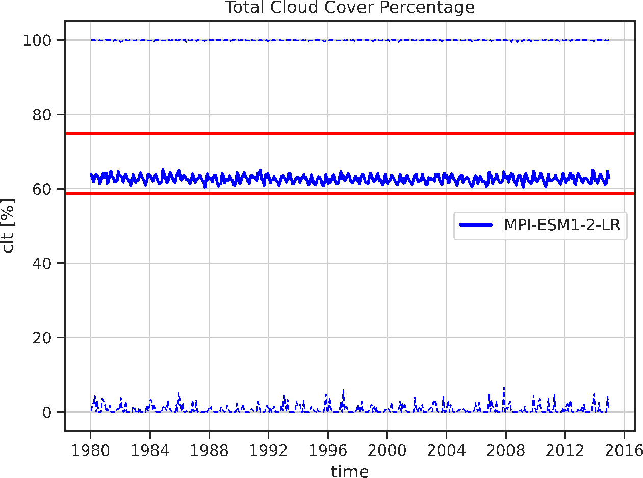
_images/timeseries_ambiguous_variable_group_MPI-ESM1-2-LR_Amon_historical_r1i1p1f1.png — Fig. 74 Time series of monthly global average (solid line) and minimum / maximum (dashed lines) total cloud …#

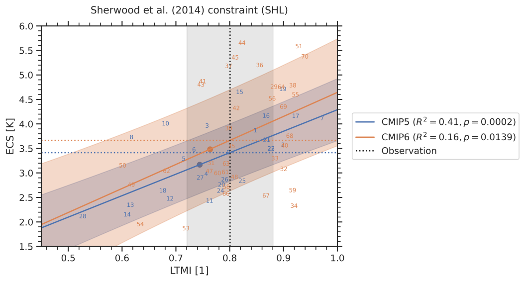
_images/SHL_scatter.png — Fig. 75 Emergent relationship (solid blue and orange lines) of the Sherwood et al. (2014) emergent constrain…#

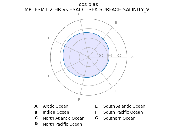
_images/radar_bias.png — Fig. 76 Radar plot showing the mean state biases (simulation minus observations) for the regional averages o…#

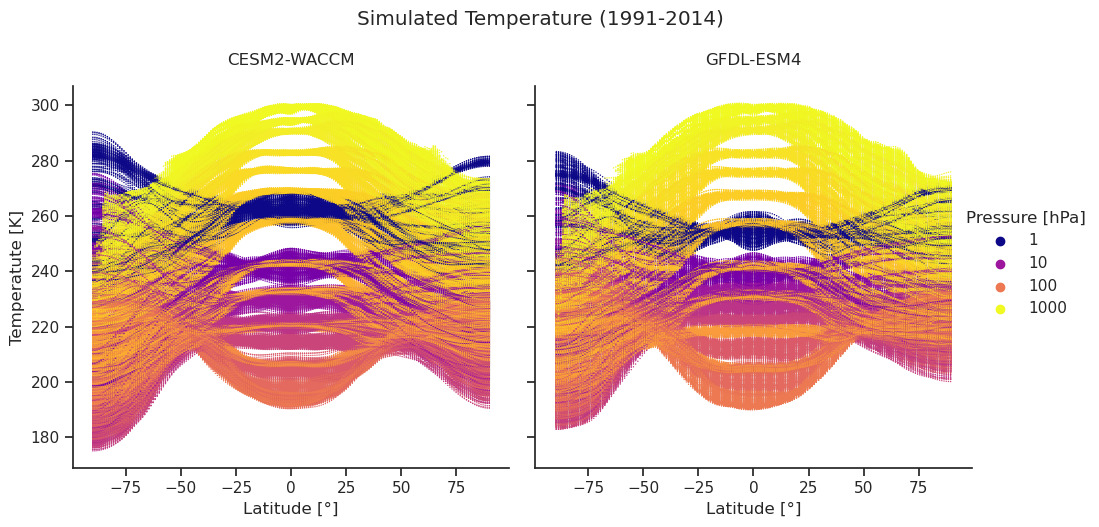
_images/ta_vs_lat.jpg — Fig. 77 Monthly and zonal mean temperatures vs. latitude in the period 1991-2014 for two Earth system models…#

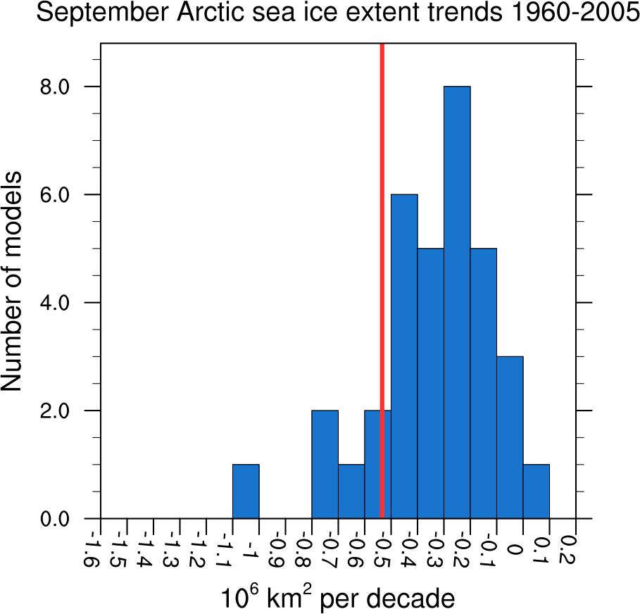
_images/trend_sic_extend_Arctic_September_histogram.png — Fig. 78 Sea ice extent trend distribution for the Arctic in September (similar to IPCC AR5 Chapter 9, Fig. 9…#

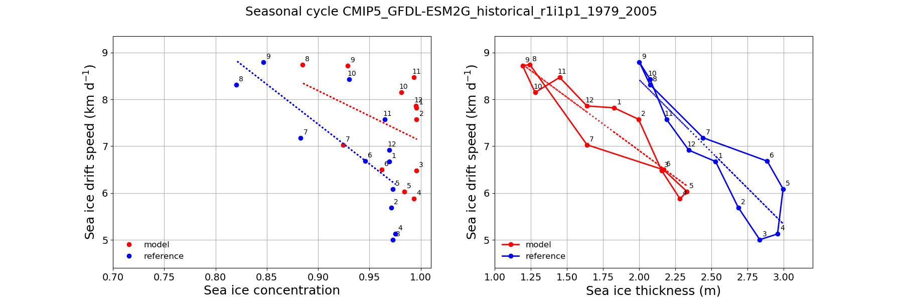
_images/drift-strength.png — Fig. 79 Scatter plots of modelled (red) and observed (blue) monthly mean sea-ice drift speed against sea-ice…#

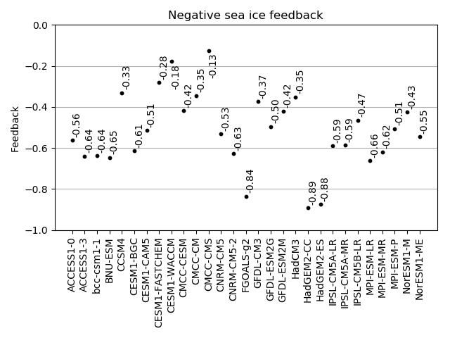
_images/negative_feedback.png — Fig. 80 Seaice negative feedback values (CMIP5 historical experiment 1979-2004).#

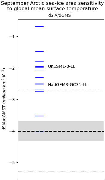
_images/September_Arctic_sea_ice_sensitivity.png — Fig. 81 Plot of sensitivity of northern hemisphere sea ice area loss (millions of square kilometres) in the …#

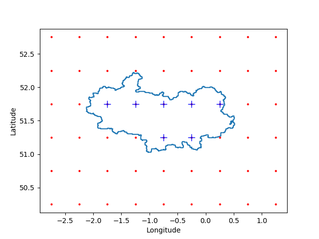
_images/shapeselect.png — Fig. 82 Example of the selection of model grid points falling within (blue pluses) and without (red dots) a …#

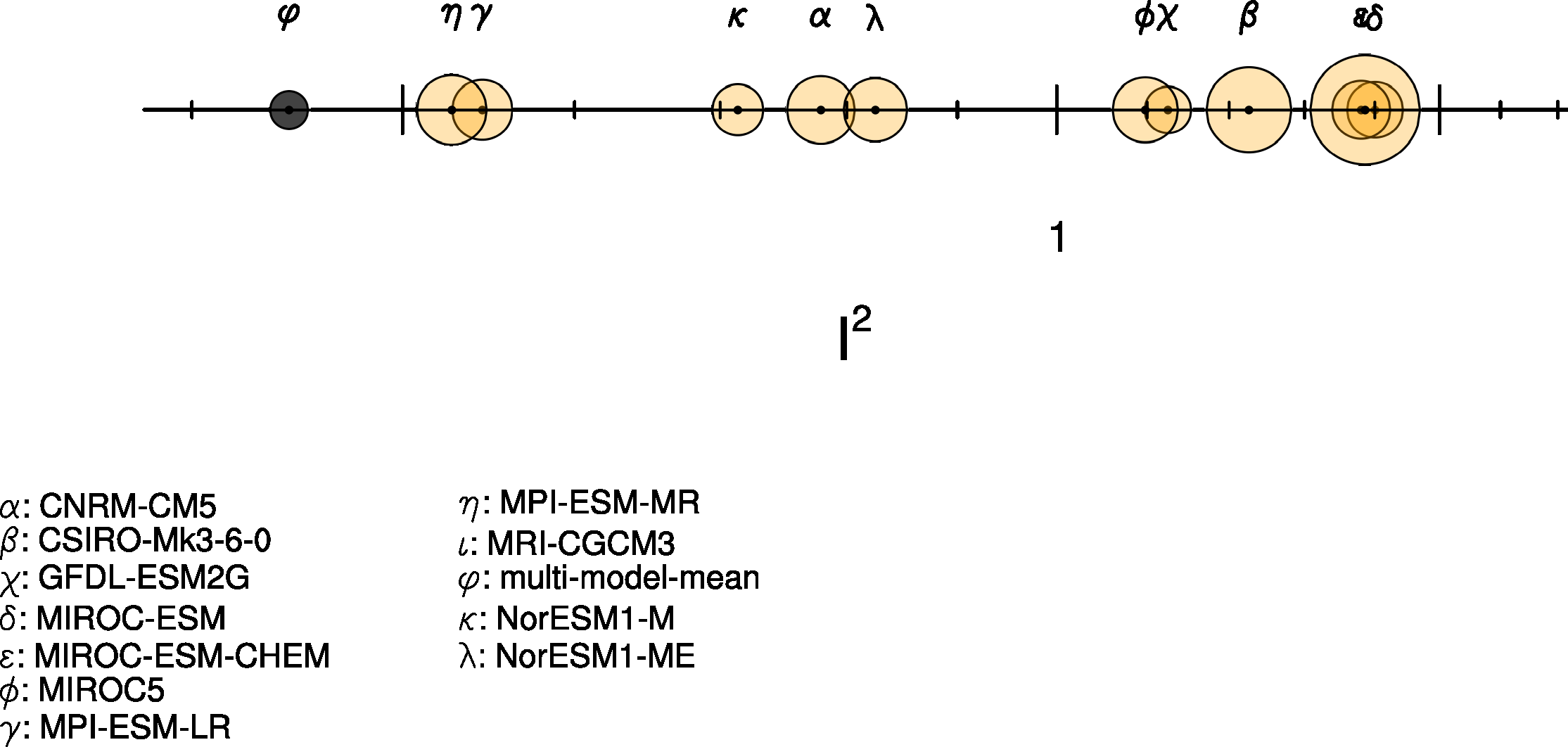
_images/reichlerkim08bams_smpi.png — Fig. 83 Performance index I2 for individual models (circles). Circle sizes indicate the length of the 95% co…#

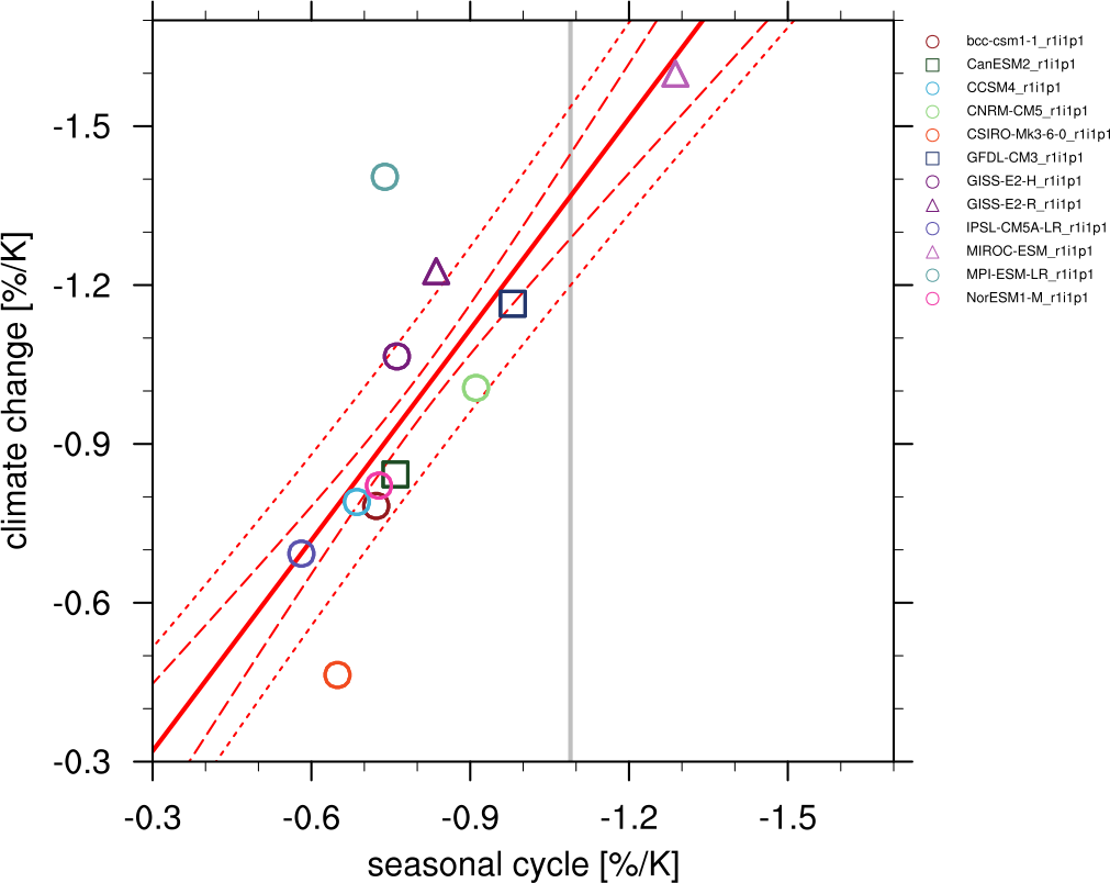
_images/fig-9-45a.png — Fig. 84 Scatterplot of springtime snow-albedo effect values in climate change vs. springtime Delta alpha_s…#

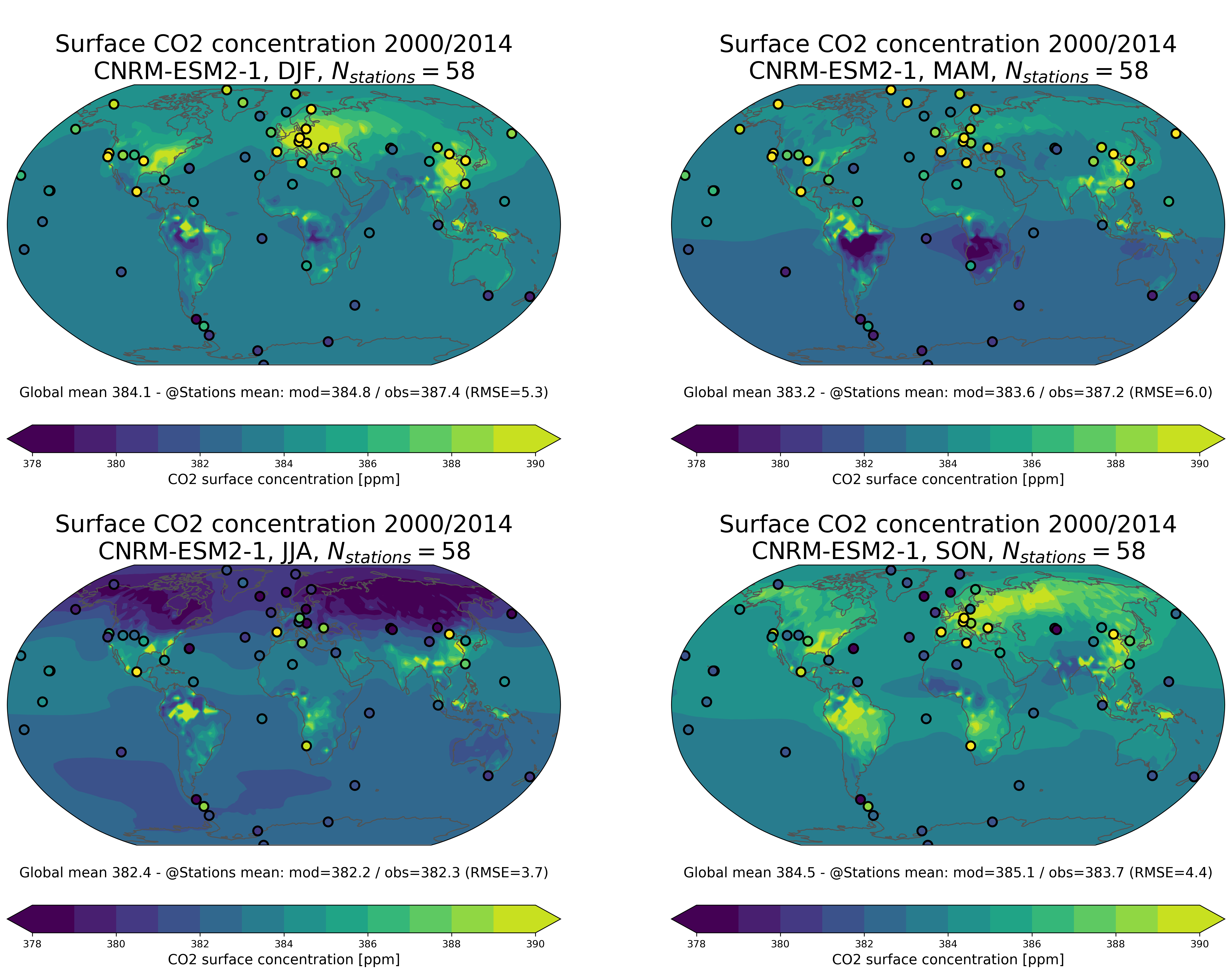
_images/CNRM-ESM2-1_Amon_esm-hist_co2s_2000_2014_seas_map.png — Fig. 85 Evaluation of seasonal surface concentration of CO2 from CNRM-ESM2-1 esm-hist member r1i1p1f3 agains…#

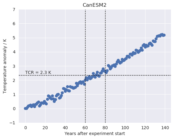
_images/CanESM21.png — Fig. 86 Time series of the global mean surface air temperature anomaly (relative to the linear fit of the pr…#

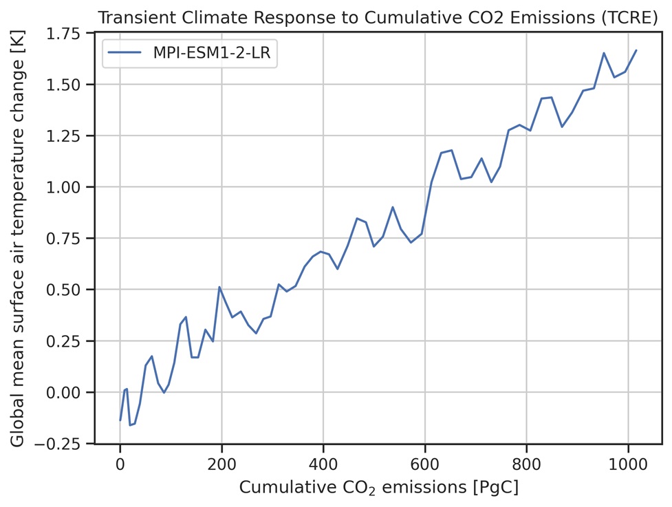
_images/tcre.jpg — Fig. 87 Global mean surface air temperature anomaly versus cumulative CO2 emissions for MPI-ESM1-2-LR using …#

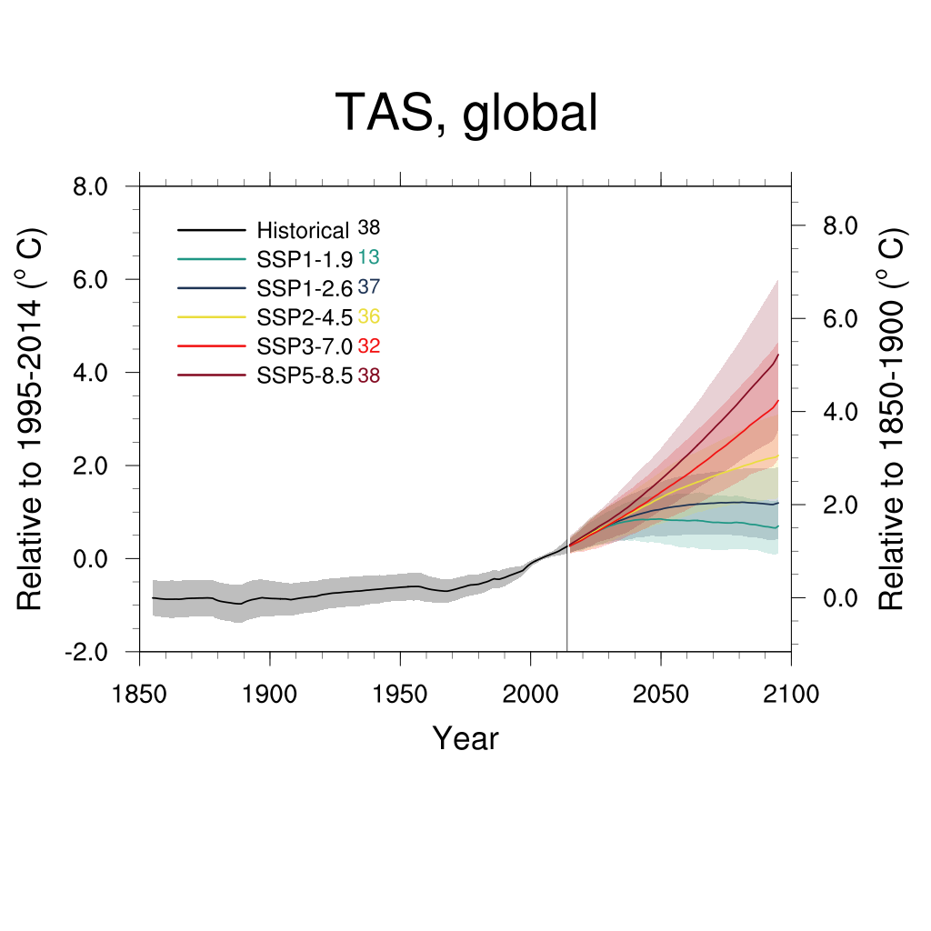
_images/tas_timeseries.png — Fig. 88 Global average temperature time series (11-year running averages) of changes from current baseline (…#

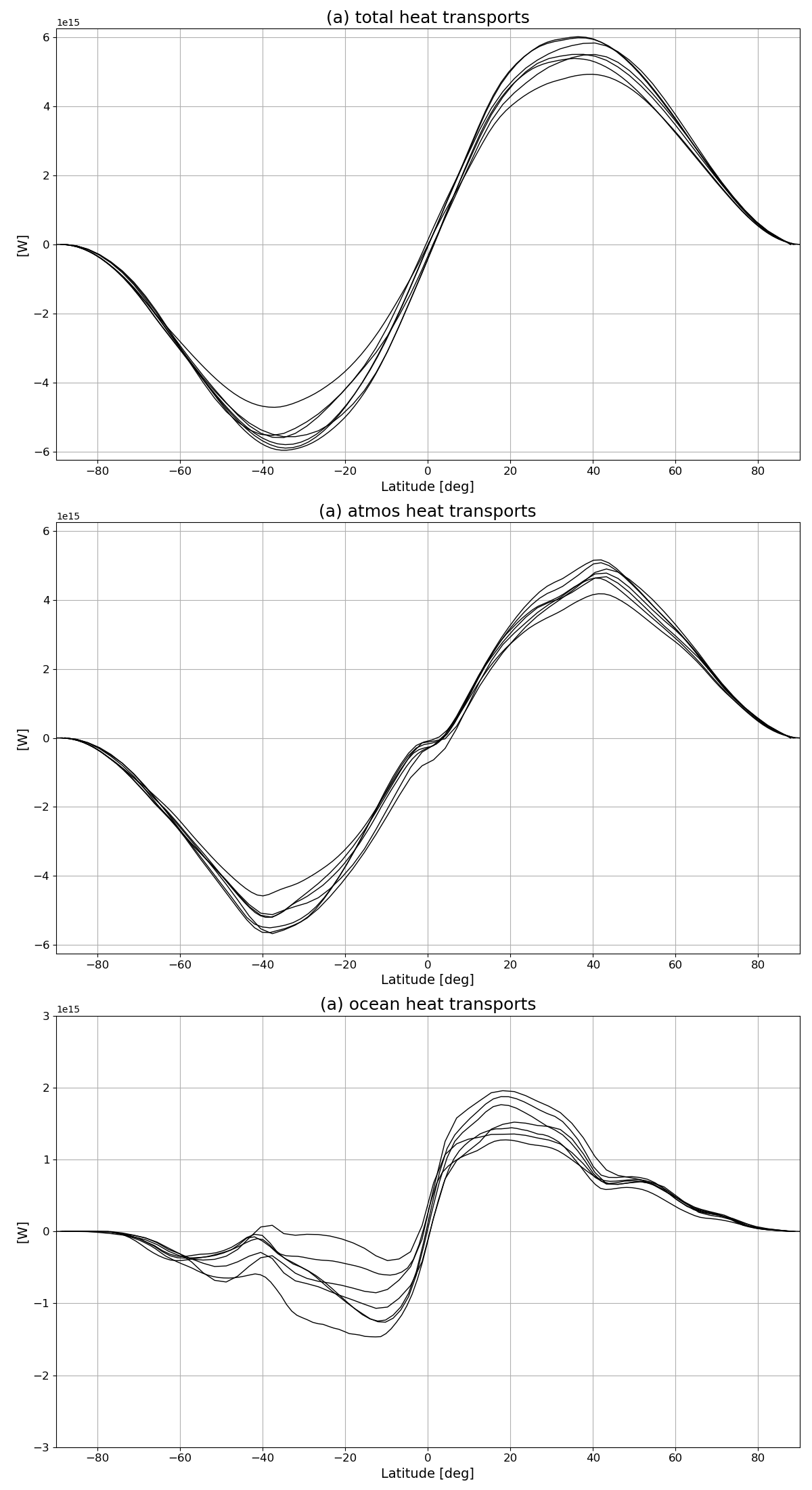
_images/meridional_transp.png — Fig. 89 Meridional transports.#

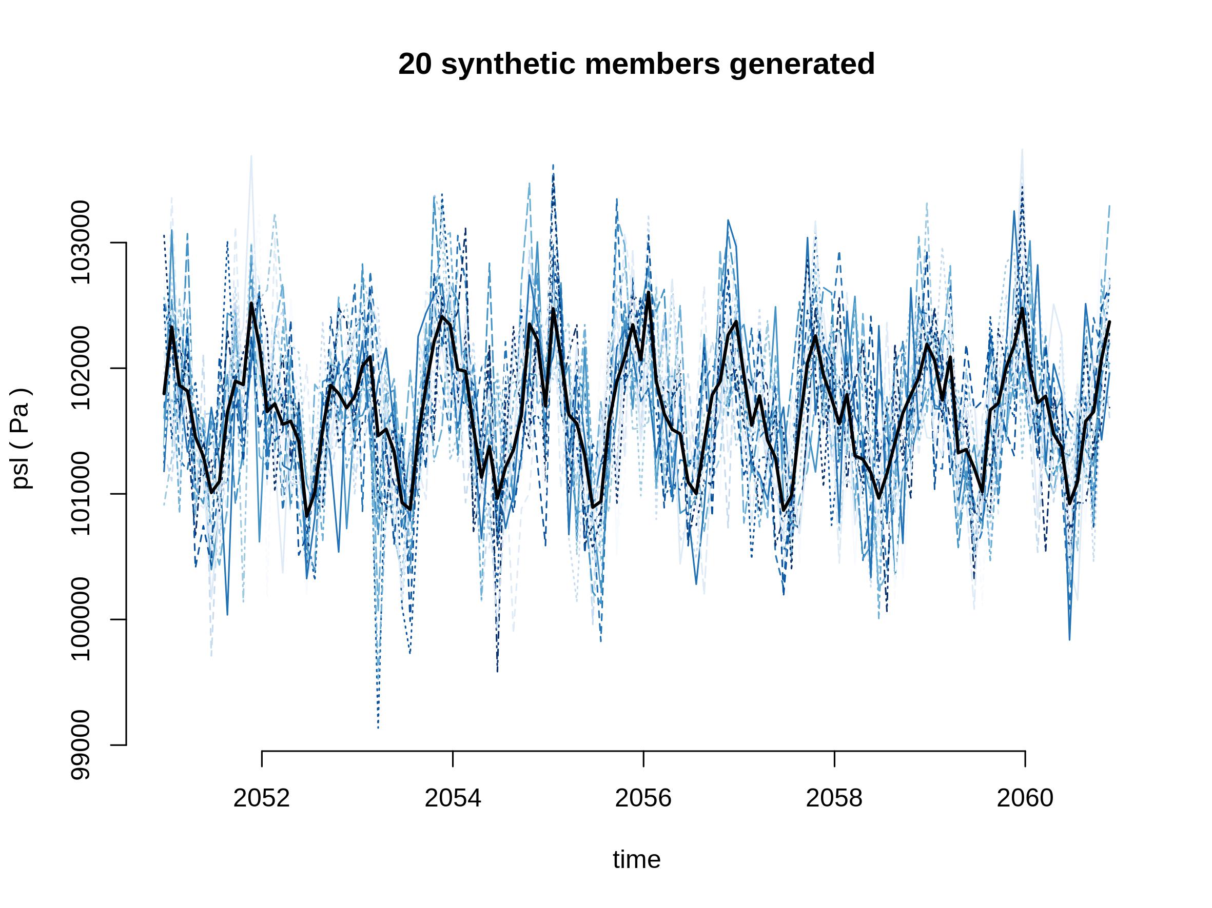
_images/synthetic_CMIP5_bcc-csm1-1_Amon_rcp45_r1i1p1_psl_2051-2060.jpg — Fig. 90 Twenty synthetic single-model ensemble generated by the recipe_toymodel.yml (see Section 3.7.2) for …#

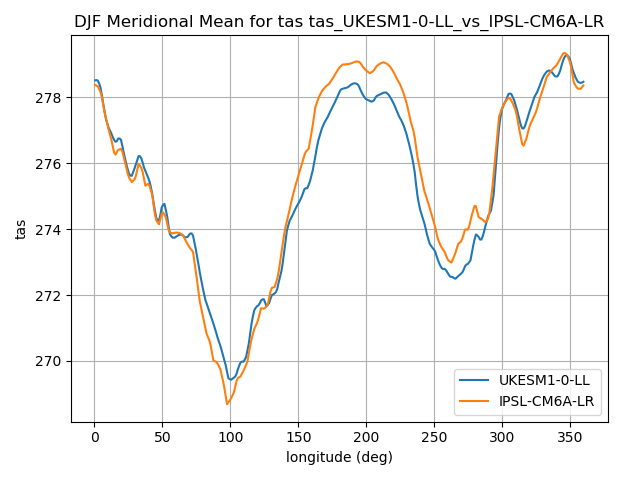
_images/Merid_Mean_DJF_longitude_tas_UKESM1-0-LL_vs_IPSL-CM6A-LR.png — Fig. 91 Meridional seasonal mean for winter (DJF) comparison beween CMIP6 UKESM1 and IPSL models.#

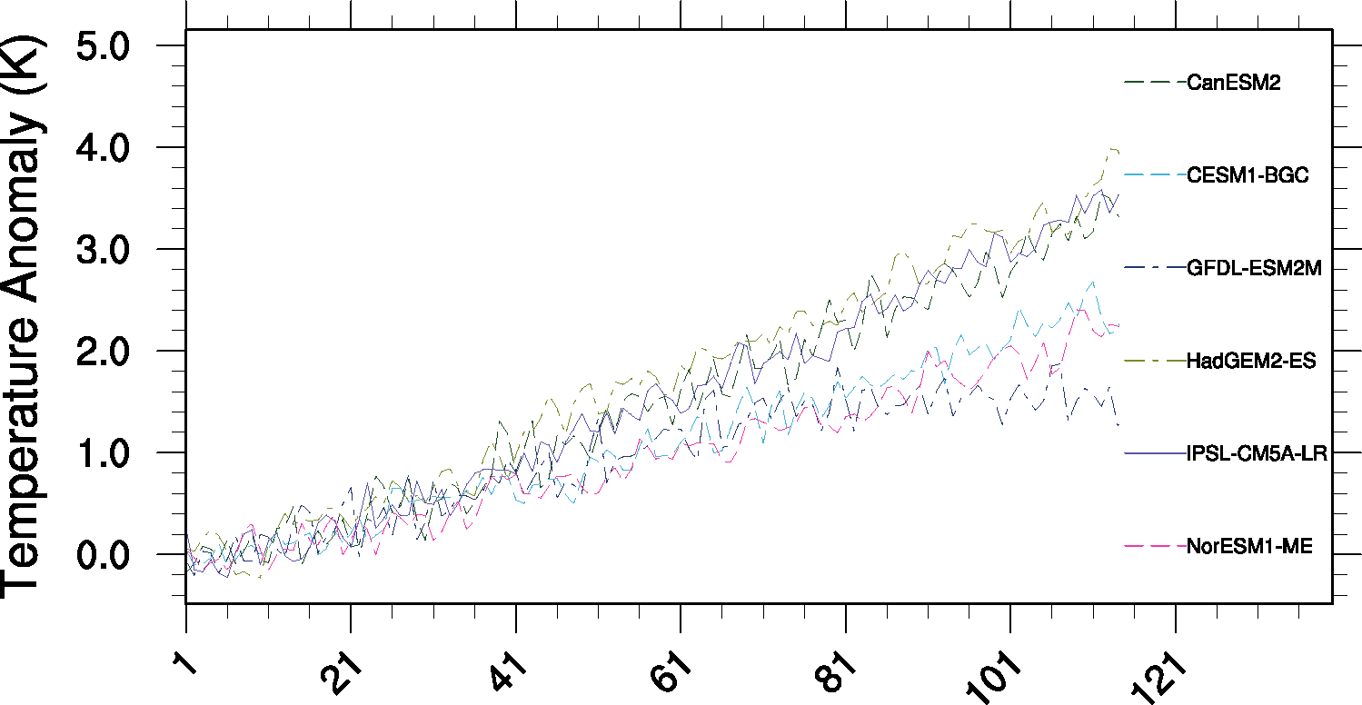
_images/tas_Global_CMIP5_1pctCO2_anom__1-1999.png — Fig. 92 Time series of tropical (30S to 30N) mean near surface temperature (tas) change between year 30 and …#

_images/CMPI5_uajet-pos_rcp45_20ystep_FIG1.png — Fig. 93 Time series of the the target variable (future austral jet position in the RCP 4.5 scenario) for the…#

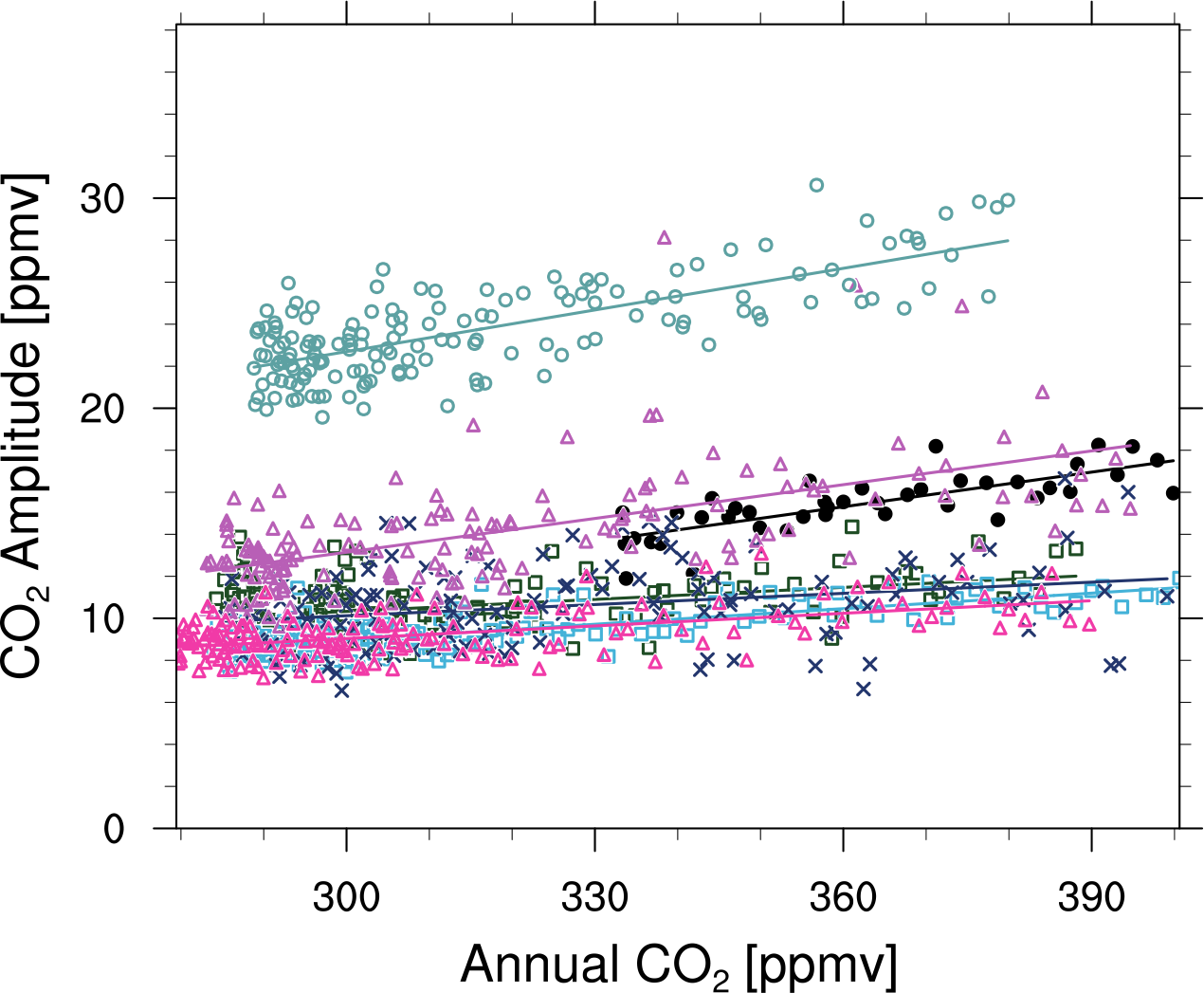
_images/fig_1.png — Fig. 94 Comparison of CO2 seasonal amplitudes for CMIP5 historical simulations and observations showing annu…#

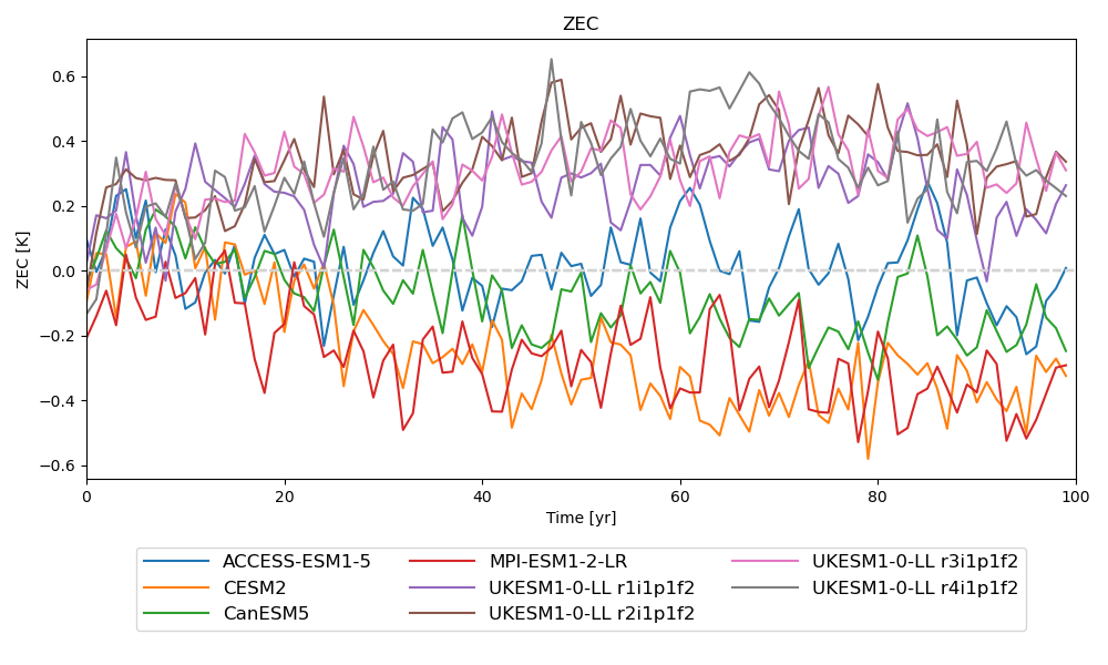
_images/zec_ts.png — Fig. 95 Time series of ZEC - temperature change after cessation of emissions.#

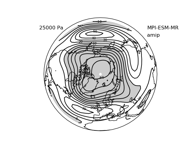
_images/zmnam_reg.png — Fig. 96 Regression map of the Northern Hemisphere zonal mean AM index onto geopotential height, for a select…#

Contact	Impressum	Terms of use	Acknowledgements
Birgit Hassler (Project Co-PI) Axel Lauer (Core Developer)	Legal Notice	Terms of use	ESMValTool Funding