Equilibrium climate sensitivity#
Overview#
Equilibrium climate sensitivity is defined as the change in global mean temperature as a result of a doubling of the atmospheric CO2 concentration compared to pre-industrial times after the climate system has reached a new equilibrium. This recipe uses a regression method based on Gregory et al. (2004) to calculate it for several CMIP models.
Available recipes and diagnostics#
Recipes are stored in recipes/
recipe_ecs.yml
Diagnostics are stored in diag_scripts/
climate_metrics/ecs.py
climate_metrics/create_barplot.py
climate_metrics/create_scatterplot.py
User settings in recipe#
Preprocessor
area_statistics(operation: mean): Calculate global mean.
Script climate_metrics/ecs.py
calculate_mmm, bool, optional (default:True): Calculate multi-model mean ECS.complex_gregory_plot, bool, optional (default:False): Plot complex Gregory plot (also add response for firstsep_yearyears and last 150 -sep_yearyears, default:sep_year=20) ifTrue.output_attributes, dict, optional: Write additional attributes to netcdf files.read_external_file, str, optional: Read ECS and feedback parameters from external file. The path can be given relative to this diagnostic script or as absolute path.savefig_kwargs, dict, optional: Keyword arguments formatplotlib.pyplot.savefig().seaborn_settings, dict, optional: Options forseaborn.set_theme()(affects all plots).sep_year, int, optional (default:20): Year to separate regressions of complex Gregory plot. Only effective ifcomplex_gregory_plotisTrue.x_lim, list of float, optional (default:[1.5, 6.0]): Plot limits for X axis of Gregory regression plot (T).y_lim, list of float, optional (default:[0.5, 3.5]): Plot limits for Y axis of Gregory regression plot (N).
Script climate_metrics/create_barplot.py
add_mean, str, optional: Add a bar representing the mean for each class.label_attribute, str, optional: Cube attribute which is used as label for different input files.order, list of str, optional: Specify the order of the different classes in the barplot by giving thelabel, makes most sense when combined withlabel_attribute.patterns, list of str, optional: Patterns to filter list of input data.savefig_kwargs, dict, optional: Keyword arguments formatplotlib.pyplot.savefig().seaborn_settings, dict, optional: Options forseaborn.set_theme()(affects all plots).sort_ascending, bool, optional (default:False): Sort bars in ascending order.sort_descending, bool, optional (default:False): Sort bars in descending order.subplots_kwargs, dict, optional: Keyword arguments formatplotlib.pyplot.subplots().value_labels, bool, optional (default:False): Label bars with value of that bar.y_range, list of float, optional: Range for the Y axis of the plot.
Script climate_metrics/create_scatterplot.py
dataset_style, str, optional: Name of the style file (located inesmvaltool.diag_scripts.shared.plot.styles_python).pattern, str, optional: Pattern to filter list of input files.seaborn_settings, dict, optional: Options forseaborn.set_theme()(affects all plots).y_range, list of float, optional: Range for the Y axis of the plot.
Variables#
rlut (atmos, monthly, longitude, latitude, time)
rsdt (atmos, monthly, longitude, latitude, time)
rsut (atmos, monthly, longitude, latitude, time)
tas (atmos, monthly, longitude, latitude, time)
Observations and reformat scripts#
None
References#
Gregory, Jonathan M., et al. “A new method for diagnosing radiative forcing and climate sensitivity.” Geophysical research letters 31.3 (2004).
Example plots#
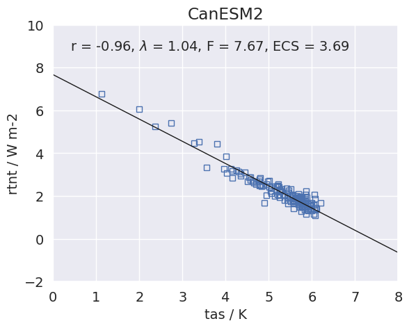
Fig. 261 Scatterplot between TOA radiance and global mean surface temperature anomaly for 150 years of the abrupt 4x CO2 experiment including linear regression to calculate ECS for CanESM2 (CMIP5).#